【AI】目标检测算法DETR源码解析及推理测试
说到目标检测,自然而然我们会想到YOLO这个框架,YOLO框架已经发展到V8版本了,各种应用也比较成熟,不过我最近在研究Transformer,今天的主角是Transformer在目标检测的开山之作:DETR:End-to-End Object Detection with Transformers,这是由Facebook AI团队出品的,其源码地址在:https://github.com/facebookresearch/detr。
0.DETR简介
DETR的特别之一在于将transformer应用于目标检测领域;而他不同于之前的算法的地方在于它不像YOLO这种使用anchor,也不想faster-rcnn使用各种proposal方法,同时它还去除了NMS,这让它在当时一众目标检测算法中显得比较特别。
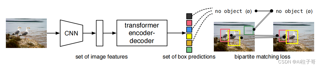
论文提出了一种将目标检测视为直接集预测问题的新方法。DETR简化了检测流程,有效地消除了对许多人工设计组件的需求,如NMS或anchor生成。新框架的主要组成部分,称为DEtection TRansformer或DETR,是一种基于集合的全局损失,通过二分匹配强制进行一对一预测,以及一种transformer encoder-decoder架构。
基本思想:
(1)先来个CNN得到各Patch作为输入,再套transformer做编码和解码;
(2)编码的路子跟VIT基本一样,重点在解码,直接预测N个坐标框(原文是100个);

(3)编码(Encoder)的主要任务是得到各个目标的注意力结果,准备好特征,等解码器来进行匹配
(4)解码(Decoder)过程的核心目标是让object queries学会从原始特征中找到物体的位置;
(5)object queries采用随机初始化的方式(0+位置编码);
(6)输出层就是N个object queries的预测;
(7)输出的匹配采用匈牙利匹配方式,按照loss最小的组合,匹配上的作为目标输出,没有匹配上的都作为背景。
DETR不仅可以用在检测领域,在分割领域也同样可用。性能上倒是还不错,就是训练太慢了,训练模型的机器配置要求也比较高。
1.源码解析
源码的启动程序是main.py程序,在main函数中,主要关注build_model和build_dataset,这两个分别是构建模型和构建数据集的。
1.1数据集处理
模型的数据集采用的coco2017,其数据集处理也是采用的coco数据集格式,对于需要使用自己数据集的,需要将图像和标注文件都做成coco数据集的形式,否则需要自己实现数据集加载的程序。运行模型训练需要指定数据集的路径,即coco_path参数。
由build_dataset函数可知,构建数据集的操作位于coco.py文件中,这里直接继承了torchvision中的方法torchvision.datasets.CocoDetection
class CocoDetection(torchvision.datasets.CocoDetection):
    def __init__(self, img_folder, ann_file, transforms, return_masks):
        super(CocoDetection, self).__init__(img_folder, ann_file)
        self._transforms = transforms
        self.prepare = ConvertCocoPolysToMask(return_masks)

    def __getitem__(self, idx):
        img, target = super(CocoDetection, self).__getitem__(idx)
        image_id = self.ids[idx]
        target = {'image_id': image_id, 'annotations': target}
        img, target = self.prepare(img, target)
        if self._transforms is not None:
            img, target = self._transforms(img, target)
        return img, target
这里数据准备用到了ConvertCocoPolysToMask函数,可以跳入进去,这里面主要对标注进行了处理,将xywh形式的标注转为x1y1x2y2的标注格式,x1y1是标注框左上角的点,x2y2是标注框右下角的点。
只保留iscrowd == 0,就是单个目标没有重叠的
anno = [obj for obj in anno if 'iscrowd' not in obj or obj['iscrowd'] == 0]
x y w h转换成了 x1y1 x2y2
boxes = [obj["bbox"] for obj in anno] # x y w h
        # guard against no boxes via resizing
        boxes = torch.as_tensor(boxes, dtype=torch.float32).reshape(-1, 4)
        boxes[:, 2:] += boxes[:, :2]
        boxes[:, 0::2].clamp_(min=0, max=w)
        boxes[:, 1::2].clamp_(min=0, max=h)
过滤掉左上角坐标小于右下角坐标的标注(注意自己标数据的时候可能出现的),这种情况是在标注数据的时候画框从右下角拉到左上角,这样容易导致错误,所以需要过滤掉。
keep = (boxes[:, 3] > boxes[:, 1]) & (boxes[:, 2] > boxes[:, 0])
1.2模型解析
模型代码总的代码位于detr.py文件,我们可以跟随DETR类的forward函数来看模型数据处理的方式:
backbone
首先经过backbone,backbone对数据进行了两个操作,获取特征图和位置编码:
features, pos = self.backbone(samples)
跟入backbone中查看:
class Joiner(nn.Sequential):
    def __init__(self, backbone, position_embedding):
        super().__init__(backbone, position_embedding)

    def forward(self, tensor_list: NestedTensor):
        print(tensor_list.tensors.shape)
        xs = self[0](tensor_list)
        out: List[NestedTensor] = []
        pos = []
        for name, x in xs.items():
            print(x.tensors.shape)
            out.append(x)
            # position encoding
            pos.append(self[1](x).to(x.tensors.dtype))

        return out, pos
这里的xs = self[0](tensor_list)采用resnet获取特征图,而self[1](x).to(x.tensors.dtype)则是为了获取位置编码,获取特征图没有特别支出,就是走了resnet模型,获取位置编码是采用的正余弦的方式进行的,其具体操作代码位于position_encoding.py文件中的PositionEmbeddingSine类:
这里的mask是将非数据的特征值去掉,位置编码采用的是在二维矩阵的行方向和列方向求cumsum累加的操作:
        mask = tensor_list.mask
        assert mask is not None
        not_mask = ~mask
        y_embed = not_mask.cumsum(1, dtype=torch.float32) #行方向累加
        x_embed = not_mask.cumsum(2, dtype=torch.float32) #列方向累加
然后执行正余弦编码操作:
        # 映射成角度
        if self.normalize:
            eps = 1e-6
            y_embed = y_embed / (y_embed[:, -1:, :] + eps) * self.scale
            x_embed = x_embed / (x_embed[:, :, -1:] + eps) * self.scale
        #奇数和偶数变换
        dim_t = torch.arange(self.num_pos_feats, dtype=torch.float32, device=x.device)
        dim_t = self.temperature ** (2 * (dim_t // 2) / self.num_pos_feats)
        #计算正余弦
        pos_x = x_embed[:, :, :, None] / dim_t
        pos_y = y_embed[:, :, :, None] / dim_t
        pos_x = torch.stack((pos_x[:, :, :, 0::2].sin(), pos_x[:, :, :, 1::2].cos()), dim=4).flatten(3)
        pos_y = torch.stack((pos_y[:, :, :, 0::2].sin(), pos_y[:, :, :, 1::2].cos()), dim=4).flatten(3)
        pos = torch.cat((pos_y, pos_x), dim=3).permute(0, 3, 1, 2)
transformer
走完backbone之后我们回到detr的forward函数中,下一步就是走transformer函数了,transformer的定义位于transformer.py文件中,可以跟随代码跳入到forward函数中:
Encoder
首先进行encoder操作:
        #首先是对特征图、位置编码和mask编码的变换操作,同时生成了query_embed用于后续的decoder操作
        bs, c, h, w = src.shape
        src = src.flatten(2).permute(2, 0, 1)
        pos_embed = pos_embed.flatten(2).permute(2, 0, 1)
        query_embed = query_embed.unsqueeze(1).repeat(1, bs, 1)
        mask = mask.flatten(1)
        tgt = torch.zeros_like(query_embed)
        memory = self.encoder(src, src_key_padding_mask=mask, pos=pos_embed)
Encoder操作主要是走transformer操作,生成QKV然后计算attention,主要的操作位于TransformerEncoderLayer类中,这里计算QKV的时候只对QK进行了操作,没有对V进行操作,同时计算attention的操作直接使用了torch提供的attention计算方式:
    def forward_post(self,
                     src,
                     src_mask: Optional[Tensor] = None,
                     src_key_padding_mask: Optional[Tensor] = None,
                     pos: Optional[Tensor] = None):
        #只有K和Q 加入了位置编码;并没有对V做
        q = k = self.with_pos_embed(src, pos)
        #两个返回值:自注意力层的输出,自注意力权重;只需要第一个
        src2 = self.self_attn(q, k, value=src, attn_mask=src_mask,
                              key_padding_mask=src_key_padding_mask)[0]
        # 执行transformer连接之类的操作
        src = src + self.dropout1(src2)
        src = self.norm1(src)
        src2 = self.linear2(self.dropout(self.activation(self.linear1(src))))
        src = src + self.dropout2(src2)
        src = self.norm2(src)
        return src
Decoder
然后进行decoder操作:
跟着源码跳入TransformerDecoderLayer类的forward函数:
首先将query添加位置编码,进行自身注意力机制计算:
#这里的tgt初始值为0,融入位置编码后输入到自注意力的multihead attention的操作中
q = k = self.with_pos_embed(tgt, query_pos)
tgt2 = self.self_attn(q, k, value=tgt, attn_mask=tgt_mask,
                              key_padding_mask=tgt_key_padding_mask)[0]
然后经过一些连接操作后进入到跟Encoder中生成的K和V的注意力计算机制,这个操作是全篇核心思想的实现,这里的attention操作也是直接使用的torch中提供的多头注意力机制计算方法。
tgt2 = self.multihead_attn(query=self.with_pos_embed(tgt, query_pos),
                                   key=self.with_pos_embed(memory, pos),
                                   value=memory, attn_mask=memory_mask,
                                   key_padding_mask=memory_key_padding_mask)[0]
然后进入一些连接等其他操作,然后输出query得到最终结果。
这里Encoder和decoder都是执行多层的。
1.3损失函数
计算损失主要有三个:分类损失、回归损失和giou。这一部分位于match.py文件中
    def forward(self, outputs, targets):
        """ Performs the matching

        Params:
            outputs: This is a dict that contains at least these entries:
                 "pred_logits": Tensor of dim [batch_size, num_queries, num_classes] with the classification logits
                 "pred_boxes": Tensor of dim [batch_size, num_queries, 4] with the predicted box coordinates

            targets: This is a list of targets (len(targets) = batch_size), where each target is a dict containing:
                 "labels": Tensor of dim [num_target_boxes] (where num_target_boxes is the number of ground-truth
                           objects in the target) containing the class labels
                 "boxes": Tensor of dim [num_target_boxes, 4] containing the target box coordinates

        Returns:
            A list of size batch_size, containing tuples of (index_i, index_j) where:
                - index_i is the indices of the selected predictions (in order)
                - index_j is the indices of the corresponding selected targets (in order)
            For each batch element, it holds:
                len(index_i) = len(index_j) = min(num_queries, num_target_boxes)
        """
        bs, num_queries = outputs["pred_logits"].shape[:2]

        # We flatten to compute the cost matrices in a batch
        out_prob = outputs["pred_logits"].flatten(0, 1).softmax(-1)  # [batch_size * num_queries, num_classes]
        out_bbox = outputs["pred_boxes"].flatten(0, 1)  # [batch_size * num_queries, 4]

        # Also concat the target labels and boxes
        tgt_ids = torch.cat([v["labels"] for v in targets])
        tgt_bbox = torch.cat([v["boxes"] for v in targets])

        # Compute the classification cost. Contrary to the loss, we don't use the NLL,
        # but approximate it in 1 - proba[target class].
        # The 1 is a constant that doesn't change the matching, it can be ommitted.
        cost_class = -out_prob[:, tgt_ids]

        # Compute the L1 cost between boxes
        cost_bbox = torch.cdist(out_bbox, tgt_bbox, p=1)

        # Compute the giou cost betwen boxes
        cost_giou = -generalized_box_iou(box_cxcywh_to_xyxy(out_bbox), box_cxcywh_to_xyxy(tgt_bbox))

        # Final cost matrix
        C = self.cost_bbox * cost_bbox + self.cost_class * cost_class + self.cost_giou * cost_giou
        C = C.view(bs, num_queries, -1).cpu()

        sizes = [len(v["boxes"]) for v in targets]
        indices = [linear_sum_assignment(c[i]) for i, c in enumerate(C.split(sizes, -1))]
        return [(torch.as_tensor(i, dtype=torch.int64), torch.as_tensor(j, dtype=torch.int64)) for i, j in indices]
2.预测
模型训练好之后可以使用模型进行预测,这一部分根据官方文档来即可,我这边简单贴一下:
准备工作:
import math

from PIL import Image
import requests
import matplotlib.pyplot as plt
%config InlineBackend.figure_format = 'retina'

import ipywidgets as widgets
from IPython.display import display, clear_output

import torch
from torch import nn
from torchvision.models import resnet50
import torchvision.transforms as T
torch.set_grad_enabled(False);

# COCO classes
CLASSES = [
    'N/A', 'person', 'bicycle', 'car', 'motorcycle', 'airplane', 'bus',
    'train', 'truck', 'boat', 'traffic light', 'fire hydrant', 'N/A',
    'stop sign', 'parking meter', 'bench', 'bird', 'cat', 'dog', 'horse',
    'sheep', 'cow', 'elephant', 'bear', 'zebra', 'giraffe', 'N/A', 'backpack',
    'umbrella', 'N/A', 'N/A', 'handbag', 'tie', 'suitcase', 'frisbee', 'skis',
    'snowboard', 'sports ball', 'kite', 'baseball bat', 'baseball glove',
    'skateboard', 'surfboard', 'tennis racket', 'bottle', 'N/A', 'wine glass',
    'cup', 'fork', 'knife', 'spoon', 'bowl', 'banana', 'apple', 'sandwich',
    'orange', 'broccoli', 'carrot', 'hot dog', 'pizza', 'donut', 'cake',
    'chair', 'couch', 'potted plant', 'bed', 'N/A', 'dining table', 'N/A',
    'N/A', 'toilet', 'N/A', 'tv', 'laptop', 'mouse', 'remote', 'keyboard',
    'cell phone', 'microwave', 'oven', 'toaster', 'sink', 'refrigerator', 'N/A',
    'book', 'clock', 'vase', 'scissors', 'teddy bear', 'hair drier',
    'toothbrush'
]

# colors for visualization
COLORS = [[0.000, 0.447, 0.741], [0.850, 0.325, 0.098], [0.929, 0.694, 0.125],
          [0.494, 0.184, 0.556], [0.466, 0.674, 0.188], [0.301, 0.745, 0.933]]


# standard PyTorch mean-std input image normalization
transform = T.Compose([
    T.Resize(800),
    T.ToTensor(),
    T.Normalize([0.485, 0.456, 0.406], [0.229, 0.224, 0.225])
])

# for output bounding box post-processing
def box_cxcywh_to_xyxy(x):
    x_c, y_c, w, h = x.unbind(1)
    b = [(x_c - 0.5 * w), (y_c - 0.5 * h),
         (x_c + 0.5 * w), (y_c + 0.5 * h)]
    return torch.stack(b, dim=1)

def rescale_bboxes(out_bbox, size):
    img_w, img_h = size
    b = box_cxcywh_to_xyxy(out_bbox)
    b = b * torch.tensor([img_w, img_h, img_w, img_h], dtype=torch.float32)
    return b

def plot_results(pil_img, prob, boxes):
    plt.figure(figsize=(16,10))
    plt.imshow(pil_img)
    ax = plt.gca()
    colors = COLORS * 100
    for p, (xmin, ymin, xmax, ymax), c in zip(prob, boxes.tolist(), colors):
        ax.add_patch(plt.Rectangle((xmin, ymin), xmax - xmin, ymax - ymin,
                                   fill=False, color=c, linewidth=3))
        cl = p.argmax()
        text = f'{CLASSES[cl]}: {p[cl]:0.2f}'
        ax.text(xmin, ymin, text, fontsize=15,
                bbox=dict(facecolor='yellow', alpha=0.5))
    plt.axis('off')
    plt.show()
首先加载预训练模型,如果本地没有训练出来,可以使用官方已经训练好的,如下:
model = torch.hub.load('facebookresearch/detr', 'detr_resnet50', pretrained=True)
model.eval();
加载图片:
url = 'http://images.cocodataset.org/val2017/000000039769.jpg'
im = Image.open(requests.get(url, stream=True).raw)
模型预测:
# mean-std normalize the input image (batch-size: 1)
img = transform(im).unsqueeze(0)

# propagate through the model
outputs = model(img)

# keep only predictions with 0.7+ confidence
probas = outputs['pred_logits'].softmax(-1)[0, :, :-1]
keep = probas.max(-1).values > 0.9

# convert boxes from [0; 1] to image scales
bboxes_scaled = rescale_bboxes(outputs['pred_boxes'][0, keep], im.size)
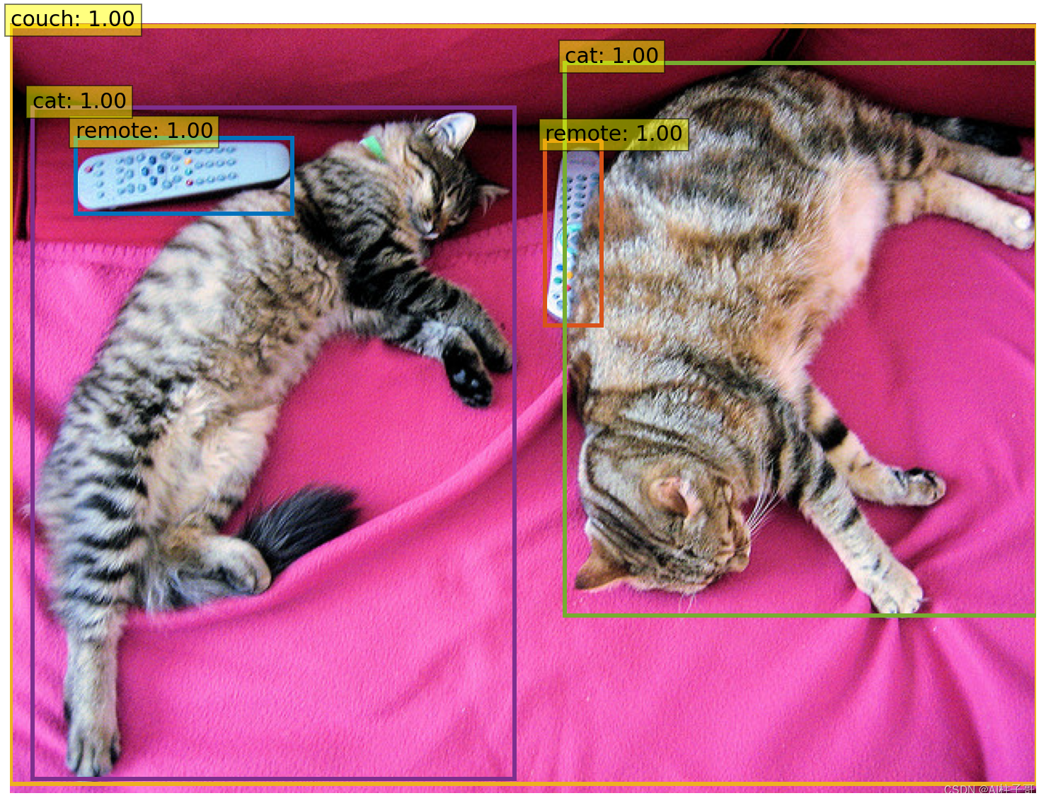
结果展示:
plot_results(im, probas[keep], bboxes_scaled)
本文来自互联网用户投稿,该文观点仅代表作者本人,不代表本站立场。本站仅提供信息存储空间服务,不拥有所有权,不承担相关法律责任。 如若内容造成侵权/违法违规/事实不符,请联系我的编程经验分享网邮箱:chenni525@qq.com进行投诉反馈,一经查实,立即删除!
- Python教程
- 深入理解 MySQL 中的 HAVING 关键字和聚合函数
- Qt之QChar编码(1)
- MyBatis入门基础篇
- 用Python脚本实现FFmpeg批量转换
- 谈谈CPU,MCU,SOC的区别和用途
- pandas字符串处理
- 开发安全之:JSON Injection
- 如何用CHAT写岗位职责概述?
- Js-基础语法(二)
- Spring Cloud Sleuth+zipkin实现链路追踪
- Leetcode的AC指南 —— 哈希法:1. 两数之和
- 汽车制动器行业调查:市场将继续呈现稳中向好发展态势
- git相关
- 甄知燕千云新版本 | 数字助理智享升级,解锁专属您的SAP/Oracle专家助理