Cell 文章图复现

多组差异火山图复现

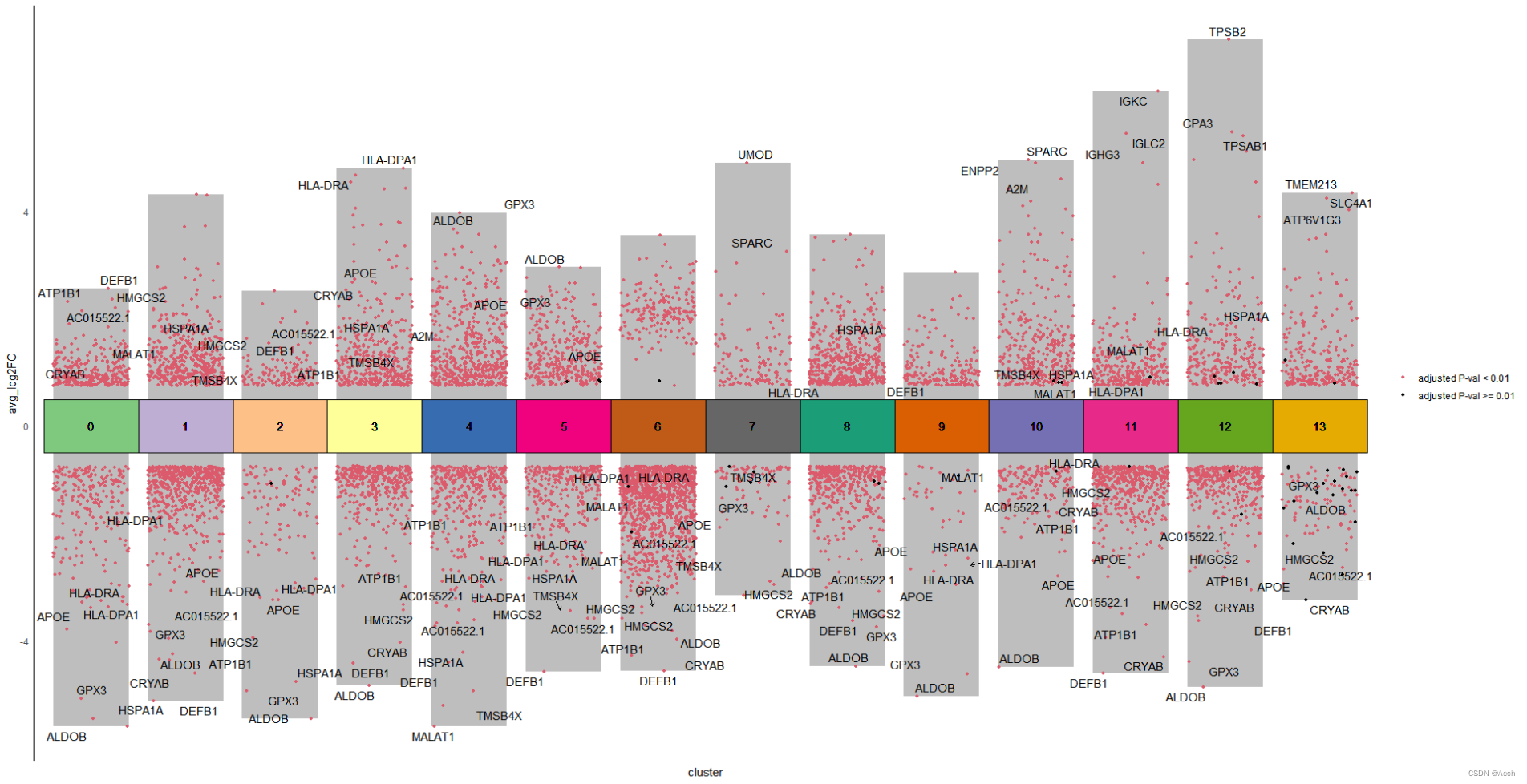
参考文章: A Spatiotemporal Organ-Wide Gene Expression and Cell Atlas of the Developing Human Heart Figure 2. H

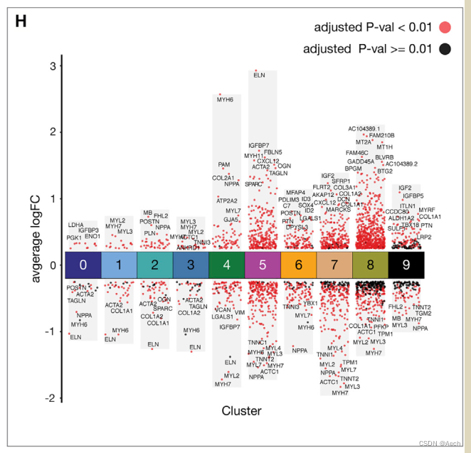
图里主要是单细胞数据不同cluster之间的差异火山图, 所以说白了就是散点图和柱状图的结合, 散点图用差异基因绘制, 柱状图利用logFC最大最小值绘制就完了.

加载包

> library(tidyverse)
> library(ggplot2)
> library(ggpubr)
> library(RColorBrewer)
> library(openxlsx)
> library(ggsci)
> library(ggrepel)
> # Create color parameters
> qual_col_pals = brewer.pal.info[brewer.pal.info$category == 'qual',]
> col_vector = unlist(mapply(brewer.pal, qual_col_pals$maxcolors, rownames(qual_col_pals)))
> 

读取数据

> deg <- read.csv("./Differentially_Expressed_Markers_Each_Cluster.csv", header = T)
> deg$cluster <- as.factor(deg$cluster)
> head(deg)
  X p_val avg_log2FC pct.1 pct.2 p_val_adj cluster       gene
1 1     0   2.558924 0.982 0.289         0       0      DEFB1
2 2     0   2.365316 0.963 0.220         0       0     HMGCS2
3 3     0   2.317304 0.991 0.513         0       0     ATP1B1
4 4     0   2.207154 0.963 0.231         0       0 AC015522.1
5 5     0   2.153153 0.912 0.244         0       0    HSD11B2
6 6     0   2.125726 0.811 0.209         0       0     PAPPA2
> deg <- deg %>% dplyr::filter(p_val_adj < 0.05) %>% 
+   dplyr::filter(abs(avg_log2FC) > 0.75) %>% 
+   dplyr::select(avg_log2FC, p_val_adj, cluster, gene)  # filter and tidy the matrix
> 

添加一些注释信息, 例如legend, 上下调, 需要显示名称的基因等

> deg <- deg %>% 
+   mutate(label = ifelse(p_val_adj < 0.01, "adjusted P-val < 0.01", "adjusted P-val >= 0.01")) %>% 
+   mutate(Change = ifelse(avg_log2FC > 0.75, "UP", "DOWN"))
> 
> bardata <- deg %>% dplyr::select(cluster, avg_log2FC ) %>% 
+   group_by(cluster) %>% 
+   summarise_all(list(tail = min, top = max)) # 
> head(bardata)
# A tibble: 6 × 3
  cluster  tail   top
  <fct>   <dbl> <dbl>
1 0       -5.61  2.56
2 1       -5.13  4.32
3 2       -5.46  2.53
4 3       -4.84  4.81
5 4       -5.60  3.97
6 5       -4.59  2.96
>
> tagedgene <- deg %>% group_by(cluster) %>% 
+   slice_max(abs(avg_log2FC), n = 3)
> head(tagedgene)
# A tibble: 6 × 6
# Groups:   cluster [2]
  avg_log2FC p_val_adj cluster gene   label                 Change
       <dbl>     <dbl> <fct>   <chr>  <chr>                 <chr> 
1      -5.61  0        0       ALDOB  adjusted P-val < 0.01 DOWN  
2      -5.46  0        0       HSPA1A adjusted P-val < 0.01 DOWN  
3      -5.09  0        0       GPX3   adjusted P-val < 0.01 DOWN  
4      -5.13  0        1       DEFB1  adjusted P-val < 0.01 DOWN  
5      -4.61  0        1       CRYAB  adjusted P-val < 0.01 DOWN  
6      -4.36  1.07e-43 1       ALDOB  adjusted P-val < 0.01 DOWN  
> 

绘制图形

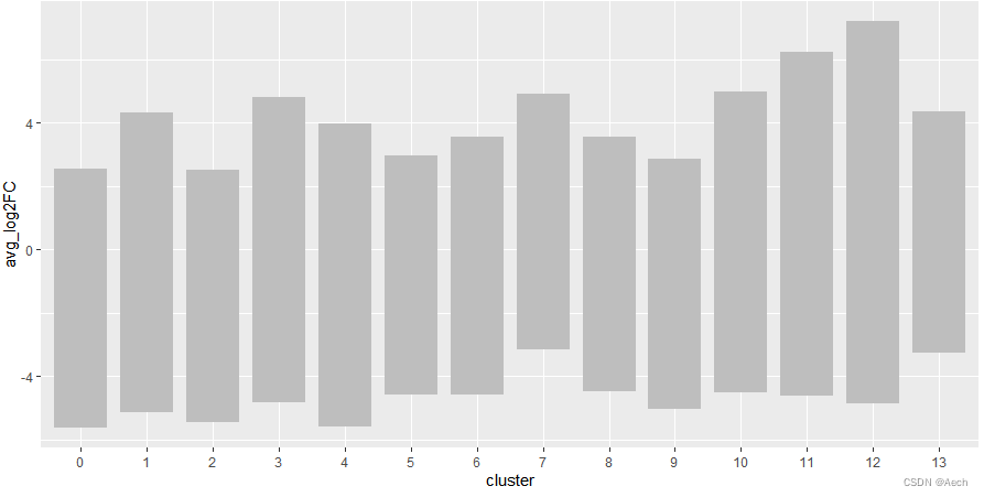
• 利用bardata绘制背景柱状图

ggplot(deg, aes(x = cluster, y = avg_log2FC ))+
  geom_col(data = bardata, mapping = aes(x = cluster, y = tail),
           fill = "grey", width = 0.8) +
  geom_col(data = bardata, mapping = aes(x = cluster, y = top),
           fill = "grey", width = 0.8)

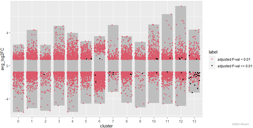
• 添加上散点图, 黑色点有点少了, 不过无所谓能看到就行

ggplot(deg, aes(x = cluster, y = avg_log2FC ))+
  geom_col(data = bardata, mapping = aes(x = cluster, y = tail),
           fill = "grey", width = 0.8) +
  geom_col(data = bardata, mapping = aes(x = cluster, y = top),
           fill = "grey", width = 0.8) +
  geom_jitter(aes(color = label), size = 1,
              position = position_jitter(seed = 0328)) +
  scale_color_manual(values = c("#db5a6b", "black"))

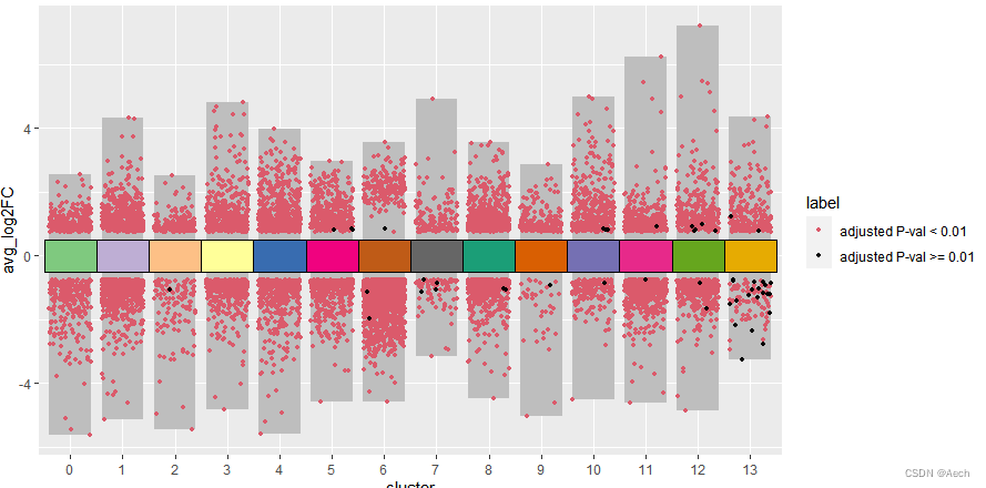
• 添加注释方块

ggplot(deg, aes(x = cluster, y = avg_log2FC ))+
  geom_col(data = bardata, mapping = aes(x = cluster, y = tail),
           fill = "grey", width = 0.8) +
  geom_col(data = bardata, mapping = aes(x = cluster, y = top),
           fill = "grey", width = 0.8) +
  geom_jitter(aes(color = label), size = 1,
              position = position_jitter(seed = 0328)) +
  scale_color_manual(values = c("#db5a6b", "black")) +
  geom_tile(aes(y = 0, fill = cluster), show.legend = F, 
            color = "black", width = 1) +
  scale_fill_manual(values = col_vector)

• 给想要展示的基因和注释方块添加文字
  • 看着有点挤, 点击zoom放大就好了

ggplot(deg, aes(x = cluster, y = avg_log2FC ))+
  geom_col(data = bardata, mapping = aes(x = cluster, y = tail),
           fill = "grey", width = 0.8) +
  geom_col(data = bardata, mapping = aes(x = cluster, y = top),
           fill = "grey", width = 0.8) +
  geom_jitter(aes(color = label), size = 1,
              position = position_jitter(seed = 0328)) +
  scale_color_manual(values = c("#db5a6b", "black")) +
  geom_tile(aes(y = 0, fill = cluster), show.legend = F, 
            color = "black", width = 1) +
  scale_fill_manual(values = col_vector) +
  geom_text(aes(y = 0, label = cluster)) +
  geom_text_repel(data = deg %>% filter(gene %in% unique(tagedgene$gene)),
                  aes(label = gene), position = position_jitter(seed = 0328),
                  arrow = arrow(angle = 30, length = unit(0.05, "inches"),
                                ends = "last", type = "open"))

• 最后处理一下背景啥的

ggplot(deg, aes(x = cluster, y = avg_log2FC ))+
  geom_col(data = bardata, mapping = aes(x = cluster, y = tail),
           fill = "grey", width = 0.8) +
  geom_col(data = bardata, mapping = aes(x = cluster, y = top),
           fill = "grey", width = 0.8) +
  geom_jitter(aes(color = label), size = 1,
              position = position_jitter(seed = 0328)) +
  scale_color_manual(values = c("#db5a6b", "black")) +
  geom_tile(aes(y = 0, fill = cluster), show.legend = F, 
            color = "black", width = 1) +
  scale_fill_manual(values = col_vector) +
  geom_text(aes(y = 0, label = cluster)) +
  geom_text_repel(data = deg %>% filter(gene %in% unique(tagedgene$gene)),
                  aes(label = gene), position = position_jitter(seed = 0328),
                  arrow = arrow(angle = 30, length = unit(0.05, "inches"),
                                ends = "last", type = "open")) +
  theme_minimal() +
  theme(axis.line.y = element_line(color = "black", linewidth = 1),
        axis.line.x = element_blank(),
        axis.text.x = element_blank(),
        panel.grid = element_blank(),
        legend.title = element_blank())

是不是很简单啊 😃
其实不只是单细胞, RNAseq等技术的差异基因也可以组合成类似的矩阵之后绘制相同的多组差异火山图. 理解这个图是柱状图和散点图的结合就可以灵活的绘制类似的图啦 😃