【图像拼接】源码精读：Perception-based seam cutting for image stitching

第一次来请先看这篇文章：【图像拼接（Image Stitching）】关于【图像拼接论文源码精读】专栏的相关说明，包含专栏内文章结构说明、源码阅读顺序、培养代码能力、如何创新等（不定期更新）

【图像拼接论文源码精读】专栏文章目录

1. 【源码精读】As-Projective-As-Possible Image Stitching with Moving DLT（APAP）第一部分：全局单应Global homography
2. 【图像拼接】源码精读：Seam-guided local alignment and stitching for large parallax images

---

前言

论文题目：Perception-based seam cutting for image stitching——基于感知的接缝剪裁图像拼接方法

论文链接：Perception-based seam cutting for image stitching

论文源码：Perception-based seam cutting for image stitching

注：matlab源码，相关算法是C++封装的。主要是对matlab的学习与理解。

论文精读：【图像拼接】论文精读：Perception-based seam cutting for image stitching

配合【论文精读】专栏对应文章阅读，效果更佳！

注：请重点关注代码段中的注释！！！有一些讲解的东西直接写在代码段的注释中了，同时多关注红色字体和绿色字体！！！

1. 跑通代码，得到结果

任何源码下载下来后，第一件事就是先跑通。

无论你是否要在该工作的基础上创新，总是需要得到拼接结果，在论文的实验部分做对比。

所以，请务必跑通，得到拼接结果。

1.1 准备工作

本地需要matlab环境，我是MATLAB R2018b，选择一个适中的matlab版本即可。（最新的matlab2023可以使用局部函数了，类似jupyter notebook，感兴趣的同学可以试试最新版。）

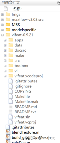
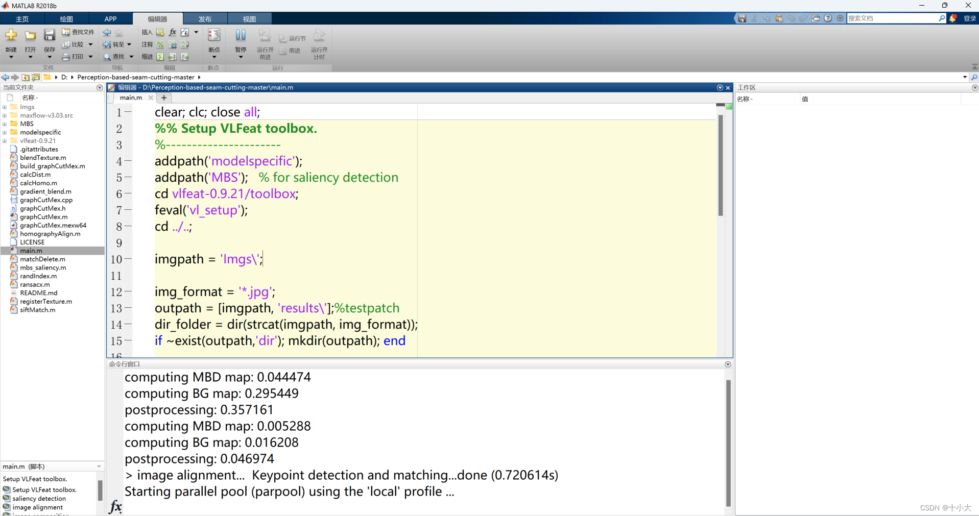
源码下载下来后，用matlab打开项目，界面如下：

左侧是文件目录结构，中级是当前所选文件代码，下面是命令行窗口，右侧是工作区（运行后显示相关变量的值）

1.2 尝试运行

点击上面菜单栏【运行】，出现如下报错：

检查后发现，vlfeat-0.9.21文件夹为空，则将其他源码中的该文件夹复制过来，同时将输入图像文件夹Imgs准备好。

vlfeat-0.9.21下载链接（已经配置好，复制到源码目录下可以直接使用）：图像拼接论文源码matlab所需的vlfeat-0.9.21库，已经配置好，复制到源码目录下即可直接使用

建议直接下载该配置好的，其他源码中的vlfeat-0.9.21可能会有报错说找不到vl_sift。

再次运行，出现如下编译错误：

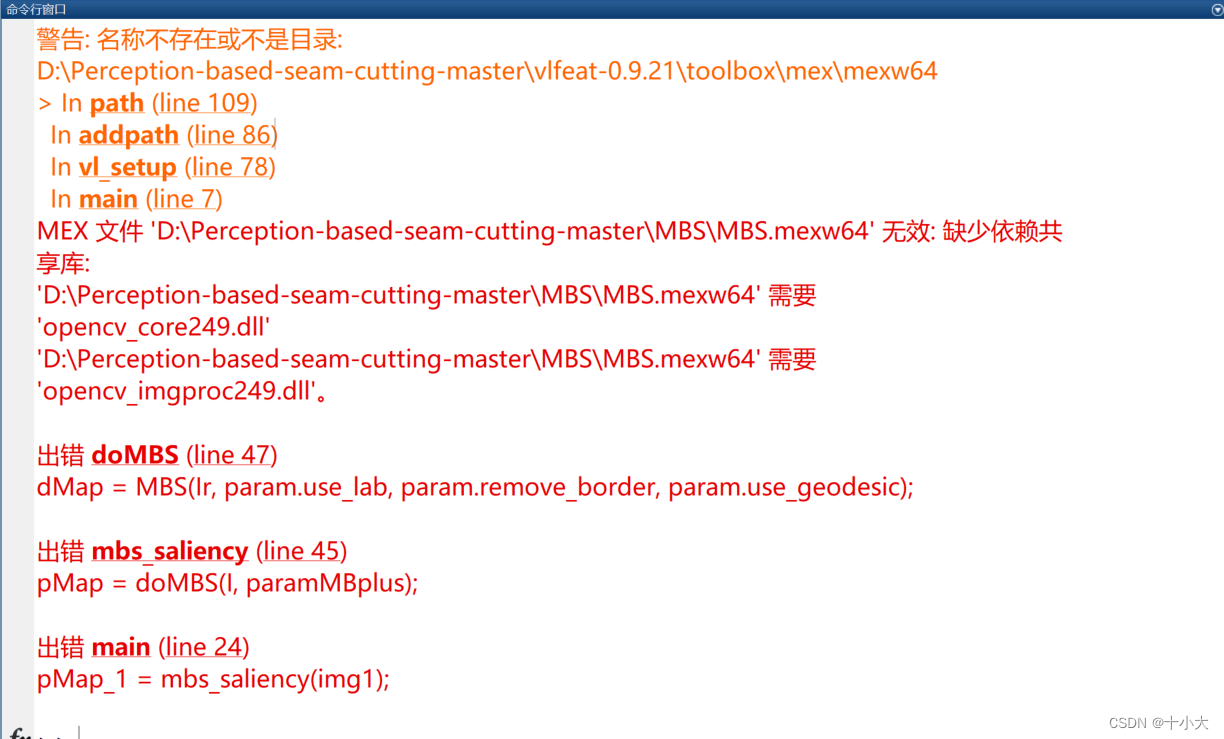
提示缺少opencv的依赖库。

解决办法1：用我自己已经编译好的MBS.mexw64配合两个opencv的dll库，下载后放到该目录中，直接解决所有的问题。（节约时间）

三个文件的下载链接：论文Perception-based seam cutting for image stitching所需的MBS依赖库

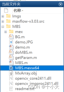
完成后直接跳过解决办法2。

解决办法2：自己一步一步编译MBS库（非常费时间，建议直接使用解决方法1，本方法可能会有其他报错）

下载opencv2.4.9：https://opencv.org/releases/page/7/

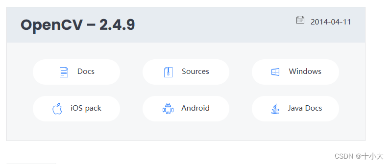
根据自己的设备，选择版本（我的是windows）。下载完毕后安装，路径为D:\opencv2.4.9即可。目的是路径位置与MBS中的路径一致：

安装完成后，会在该路径下看见上面报错的两个库文件：

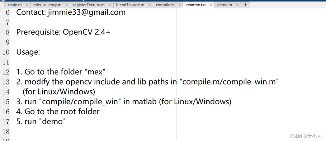
除了补充opencv的库文件外，上述报错的深层含义是我们需要提前编译好MBS中的.cpp文件，具体查看MBS中的readme：

我们将matlab的路径前进到MBS文件夹，然后执行compile.m：

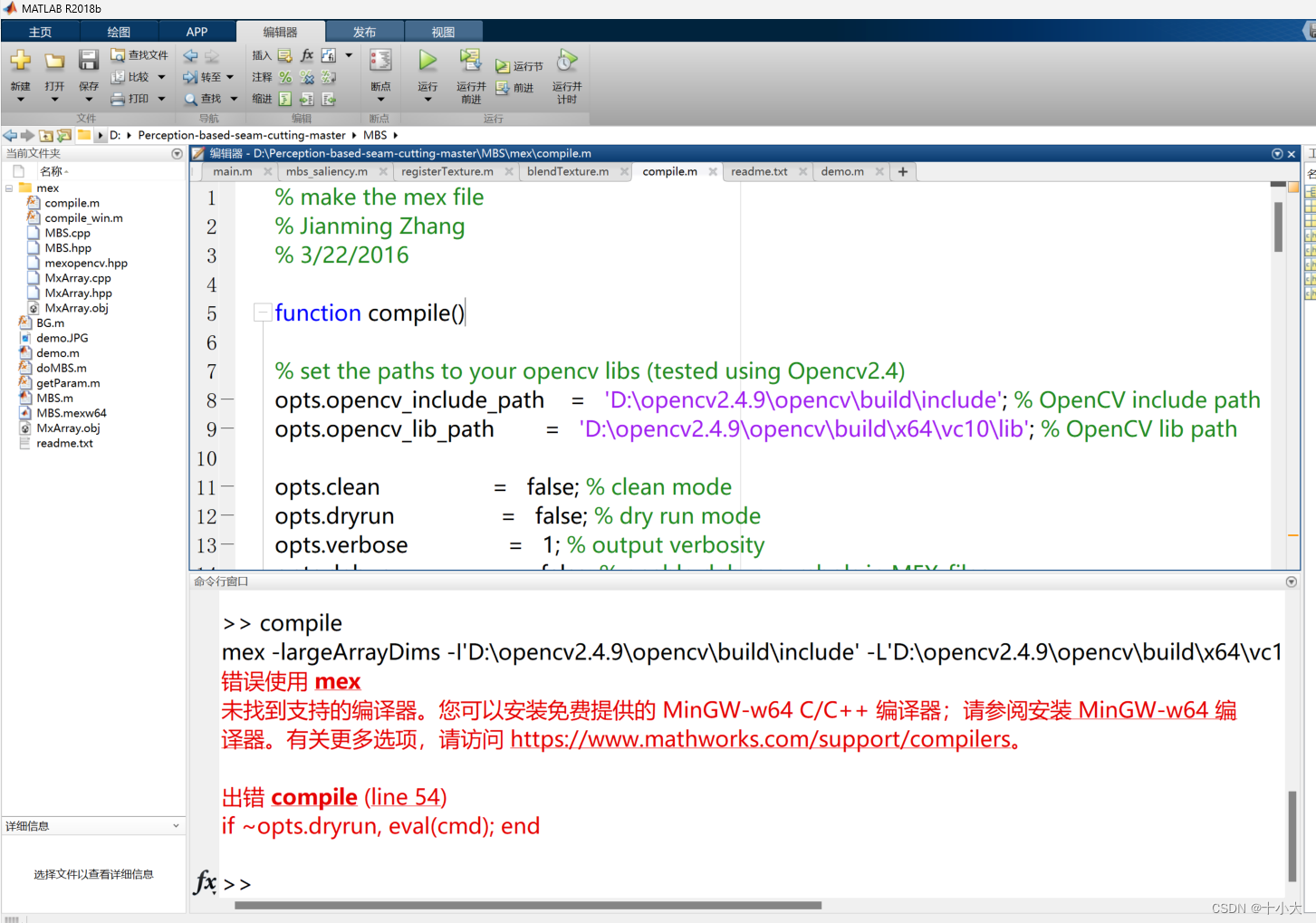
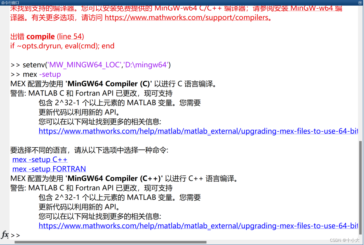
如果出现上述错误，说明你的电脑中没有该编译器，此时有两种方式解决：

1. 安装VS。如果你有C/C++需求的话，这么做最简单。
2. 单独安装MinGW-w64。

第2种方式的安装包下载地址：添加链接描述

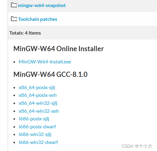
选择【x86_64-win32-seh】压缩包。（直接下载安装包会有安装错误！！！）

下载完成后，解压到D盘，目录为：D:\mingw64。

将其添加到环境变量中：

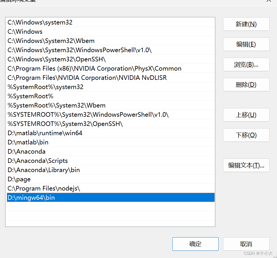
在matlab命令行输入：setenv('MW_MINGW64_LOC','D:\mingw64')和mex -setup，选择C++。

运行compile.m编译MBS，编译完成后，运行demo.m测试MBS是否有效果：

此时，MBS编译完成。再回到主目录运行main.m，代码已经可以完整的跑通了。

1.3 得到拼接结果

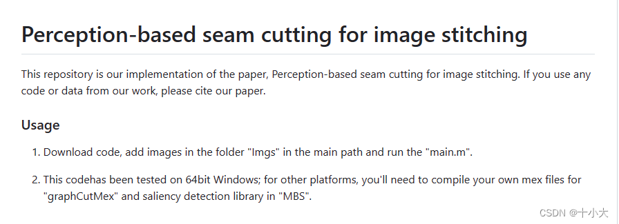
附上原作者README中的使用方法：

2. 源码解读，看懂原理

本节将按照main.m中的代码顺序进行【模块化】讲解，包括与论文中的算法对应、matlab语法和函数学习、变量的类型和值、函数功能等方面。代码段中包含原作者的注释和我做的注释，与讲解结合着阅读。

2.1 参数与输入图像

代码如下：

clear; clc; close all; 
%% Setup VLFeat toolbox.
%----------------------
addpath('modelspecific'); 
addpath('MBS');   % for saliency detection
cd vlfeat-0.9.21/toolbox;
feval('vl_setup');
cd ../..;

imgpath = 'Imgs\';
img_format = '*.jpg';
outpath = [imgpath, 'results\'];%testpatch
dir_folder = dir(strcat(imgpath, img_format));
if ~exist(outpath,'dir'); mkdir(outpath); end

path1 =  sprintf('%s%s',imgpath, dir_folder(1).name); %
path2 =  sprintf('%s%s',imgpath, dir_folder(2).name); %
img1 = im2double(imread(path1));  % target image
img2 = im2double(imread(path2));  % reference image

2.2 显著性检测

代码如下：

%% saliency detection

pMap_1 = mbs_saliency(img1);
pMap_2 = mbs_saliency(img2);

对两张输入图像进行显著性检测。

2.2.1 mbs_saliency函数

略。论文Minimum Barrier Salient Object Detection at 80 FPS详解。

2.2.2 添加可视化代码

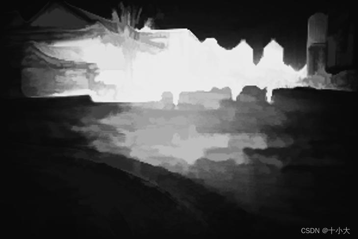
我们添加可视化代码，显示显著性检测结果：

figure,imshow(pMap_1);
title('Saliency detection for img1');
outpathfile = 'Saliency detection for img1.jpg';
imwrite(pMap_1,[outpath,outpathfile]);
figure,imshow(pMap_2);
title('Saliency detection for img2');
outpathfile = 'Saliency detection for img2.jpg';
imwrite(pMap_2,[outpath,outpathfile]);

得到两张图像的显著性检测结果：

2.3 图像对齐

main.m中的代码：

%% image alignment
fprintf('> image alignment...');tic;
[warped_img1, warped_pmap1, warped_img2, warped_pmap2] = registerTexture(img1, pMap_1, img2, pMap_2, imgpath);
fprintf('done (%fs)\n', toc);

2.3.1 registerTexture函数

function [warped_img1, warped_pmap1, warped_img2, warped_pmap2] = registerTexture(img1, pmap1, img2, pmap2, txtpath)
% given two images（img1 target， img2 reference），
% detect and match sift features, estimate homography transformation
% and calculate alignment result
% 函数功能：根据两幅原图和两幅显著图对齐纹理
% 输入：图1，显著图1，图2，显著图2，图像路径
% 输出：单应变换后的四个图

[pts1, pts2] = siftMatch(img1, img2);  
Sz1 = max(size(img1,1),size(img2,1)); % to avoid the two images have different resolution
Sz2 = max(size(img1,2),size(img2,2));
[matches_1, matches_2] = matchDelete(pts1, pts2, Sz1, Sz2); % delete wrong match features

f = figure;
imshow([img2 img1],'border','tight');
hold on;
plot(matches_2(1,:),matches_2(2,:),'go','LineWidth',2);
plot(matches_1(1,:)+size(img2,2),matches_1(2,:),'go','LineWidth',2);
plot([matches_2(1,:);matches_1(1,:)+size(img2,2)],[matches_2(2,:);matches_1(2,:)],'g-');


init_H = calcHomo(matches_1, matches_2);  % fundamental homography

[warped_img1, warped_pmap1, warped_img2, warped_pmap2] = homographyAlign(img1, pmap1, img2, pmap2, init_H);

end

其中，SIFT检测特征点函数siftMatch、RANSAC剔除异常值函数matchDelete、计算单应矩阵函数calcHomo、根据单应对齐函数homographyAlign与Seam-guided local alignment and stitching for large parallax images和Quality evaluation-based iterative seam estimation for image stitching两篇论文源码中的函数几乎一致，可以去看另外两篇源码精读，本文略。

我们在其中添加了对应匹配点的可视化，结果如下：

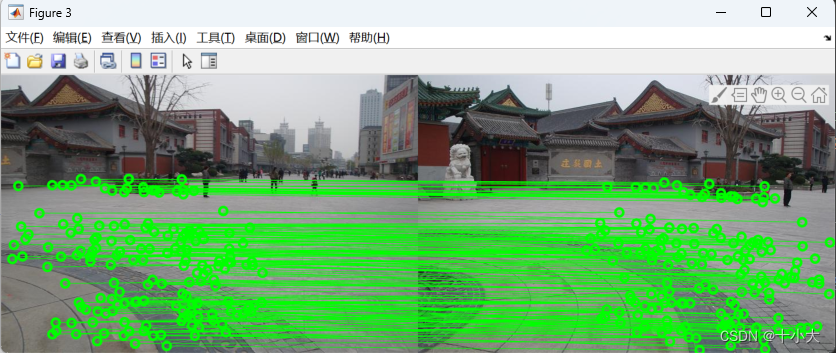
在main.m中的图像对齐代码段末尾，添加如下可视化代码：

figure,imshow(warped_img1);
title('warped_img1');
outpathfile = 'warped_img1.jpg';
imwrite(warped_img1,[outpath,outpathfile]);
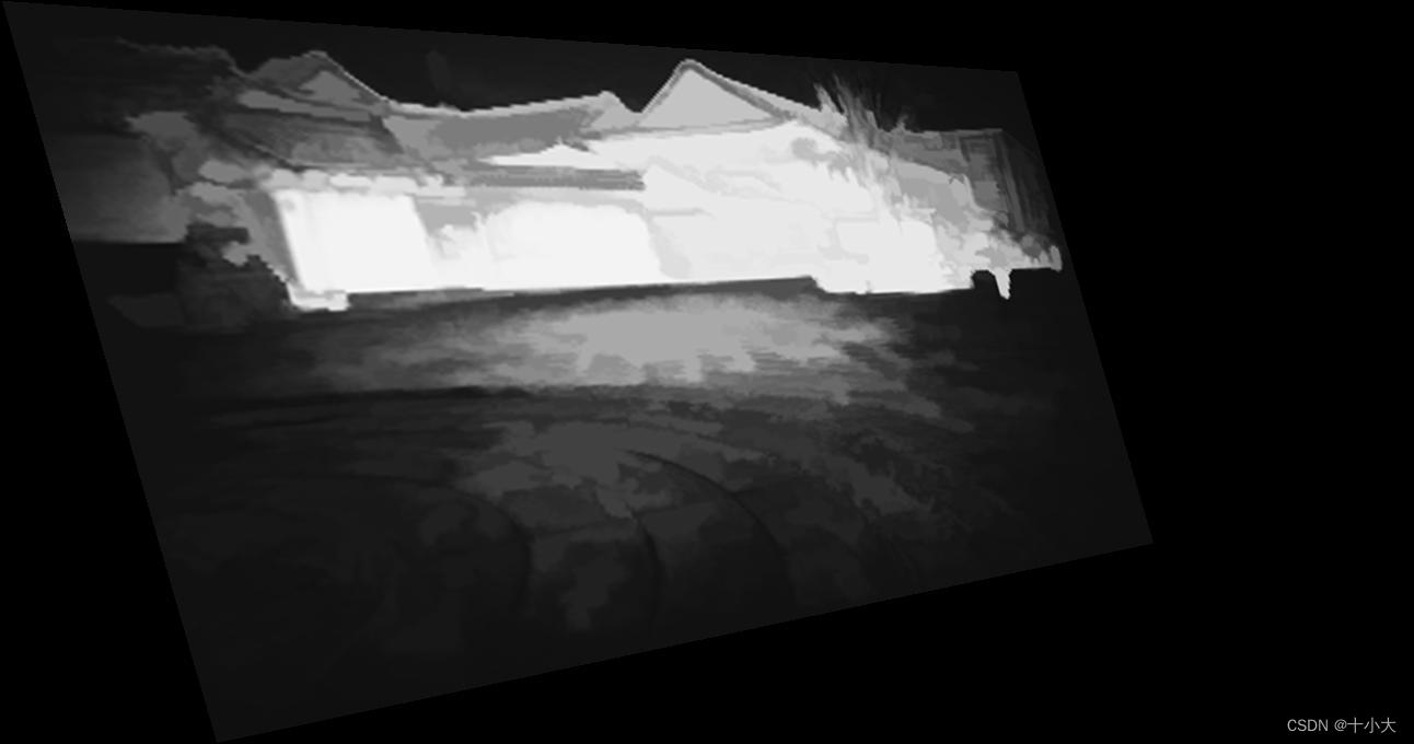
figure,imshow(warped_pmap1);
title('warped_pmap1');
outpathfile = 'warped_pmap1.jpg';
imwrite(warped_pmap1,[outpath,outpathfile]);
figure,imshow(warped_img2);
title('warped_img2');
outpathfile = 'warped_img2.jpg';
imwrite(warped_img2,[outpath,outpathfile]);
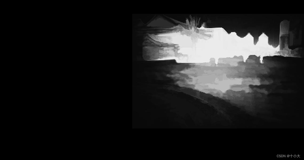
figure,imshow(warped_pmap2);
title('warped_pmap2');
outpathfile = 'warped_pmap2.jpg';
imwrite(warped_pmap2,[outpath,outpathfile]);

翘曲对齐后的原图像与显著图：

2.4 接缝融合，blendTexture函数

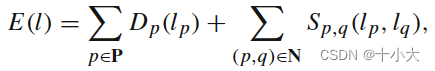
本文2.4.2中的数据项，对应论文2.1中的数据项公式（2）

本文2.4.3中的平滑项（欧氏准则），对应论文2.1中的平滑项公式（3）

本文2.4.3中的平滑项（sigmoid准则），对应论文2.2.1 中的平滑项公式（6）

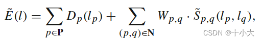
本文2.4.3中的平滑项的显著性权重，对应论文2.2.2 中的公式（8）；即最终的能量函数（论文中公式（9））由本节代码中的【数据项+显著权重*sigmoid准则下的平滑项】实现。

代码如下：

%% image composition
fprintf('> seam cutting...');tic;
imgout = blendTexture(warped_img1, warped_pmap1, warped_img2, warped_pmap2);
fprintf('done (%fs)\n', toc);

2.4.1 预处理

    % img1Homo：aligned target image
    % pmap1Homo: salient target image
    % img2Homo：aligned reference image
    % pmap2Homo: salient reference image

    %%  pre-process of blendtexture
    w1 = imfill(imbinarize(rgb2gray(warped_img1), 0),'holes');
    w2 = imfill(imbinarize(rgb2gray(warped_img2), 0),'holes');
    A = w1;  B = w2;
    C = A & B;  % mask of overlapping region
    [ sz1, sz2 ]=size(C); % 
    ind = find(C);  % index of overlapping region
    nNodes = size(ind,1); %重叠区域索引1列
    revindC = zeros(sz1*sz2,1);%每个像素值先置为0
    revindC(C) = 1:length(ind); %循环变量1到像素个数
    
    [m,~] = find(C); 
    minrow = min(m); %索引最小，最大行
    maxrow = max(m);

2.4.2 找到重叠区域边界并得到数据项

%%  terminalWeights, choose source and sink nodes
% 选择源点和汇点，一个不错的找重叠区域边界的方法

    % border of overlapping region 图2
    BR=(B-[B(:,2:end) false(sz1,1)])>0;     %重叠区域右边界(范围，是矩形)
    BL=(B-[false(sz1,1) B(:,1:end-1)])>0;   %重叠区域左边界
    BD=(B-[B(2:end,:);false(1,sz2)])>0;      %重叠区域下边界
    BU=(B-[false(1,sz2);B(1:end-1,:)])>0;   %重叠区域上边界

    CR=(C-[C(:,2:end) false(sz1,1)])>0; %图1
    CL=(C-[false(sz1,1) C(:,1:end-1)])>0;
    CD=(C-[C(2:end,:);false(1,sz2)])>0;
    CU=(C-[false(1,sz2);C(1:end-1,:)])>0;
    
    %左图重叠区域的边界(重叠区域右侧，真实边界，红色边界)
    imgseedR=(BR|BL|BD|BU)&(CR|CL|CD|CU); %RED
    imgseedB = (CR|CL|CD|CU) & ~imgseedR; %BLUE
    
    % data term 
    tw=zeros(nNodes,2);
    tw(revindC(imgseedB),2)=inf; %蓝色对应像素索引，将tw第二列设置为inf
    tw(revindC(imgseedR),1)=inf;

    mask=~(imgseedB | imgseedR); %掩码 重叠区域边界为0
    
    imglap = 0.5.*imadd(warped_img1.*cat(3,mask&C,mask&C,mask&C), warped_img2.*cat(3,mask&C,mask&C,mask&C));
%     imglap = 1.*imadd(warped_img1.*cat(3,mask&C,mask&C,mask&C), warped_img2.*cat(3,mask&C,mask&C,mask&C));
    freeseed = imgseedR;
    freeseed(minrow,:) = 0;
    freeseed(maxrow,:) = 0;
    free_seed = imgseedR & (~freeseed);
    % saliency weights
    %======================
    tw(revindC(free_seed),1) = 0;
    tw(revindC(free_seed),2) = 0;
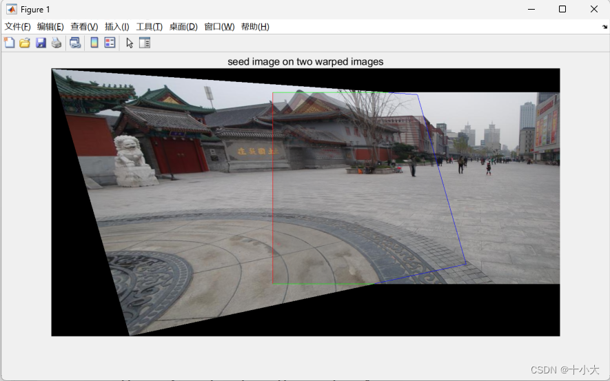
    imgseed = warped_img1.*cat(3,A-C,A-C,A-C) + warped_img2.*cat(3,B-C,B-C,B-C) + imglap+cat(3,freeseed,free_seed,imgseedB);
    %======================
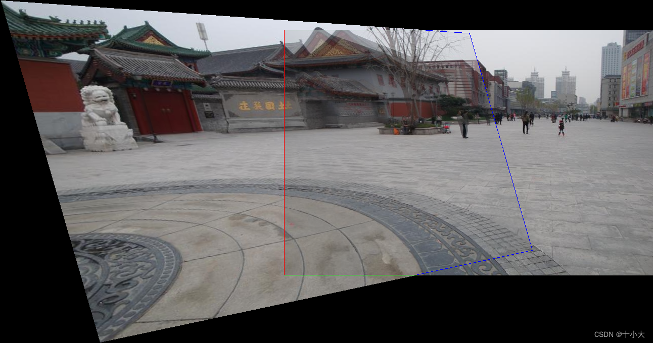
    figure,imshow(imgseed);
    title('seed image on two warped images');
    terminalWeights=tw;       % data term
    pngout = sprintf('Overlapping_result.png'); 
    imwrite(imgseed,pngout);

重叠区域可视化：

2.4.2 计算权重并得到平滑项（本文核心）

%% calculate edgeWeights

    CL1=C&[C(:,2:end) false(sz1,1)];
    CL2=[false(sz1,1) CL1(:,1:end-1)];
    CU1=C&[C(2:end,:);false(1,sz2)];
    CU2=[false(1,sz2);CU1(1:end-1,:)];
    blurred1 = warped_img1; blurred2 = warped_img2;  

	
	%  edgeWeights:  Euclidean or sigmoid or saliency-weighted sigmoid norm
	% 论文2.1
    ang_1=blurred1(:,:,1); sat_1=blurred1(:,:,2); val_1=blurred1(:,:,3);
    ang_2=blurred2(:,:,1); sat_2=blurred2(:,:,2); val_2=blurred2(:,:,3);
    % baseline difference map
    imgdif = sqrt( ( (ang_1.*C-ang_2.*C).^2+(sat_1.*C-sat_2.*C).^2+ (val_1.*C-val_2.*C).^2 )./3);
    
    % 论文2.2.1 
    % sigmoid-metric difference map
    a_rgb = 0.06; % bin of histogram
    beta=4/a_rgb; % beta
    gamma=exp(1); % base number
    para_alpha = histOstu(imgdif(C), a_rgb);  % parameter:tau
    imgdif_sig = 1./(1+power(gamma,beta*(-imgdif+para_alpha))); %公式（5） difference map with logistic function
    imgdif_sig = imgdif_sig.*C;   % difference to compute the smoothness term 
    
    % saliency-weighted sigmoid difference map
    saliency_map = ((warped_pmap1 + warped_pmap2)./2).*C;  % the saliency of overlapping region
    imgdif_sal = imgdif_sig.*(1 + saliency_map); %公式（8） difference to compute the smoothness term
    % saliency-weighted sigmoid method
    DL = (imgdif_sal(CL1)+imgdif_sal(CL2))./2;
    DU = (imgdif_sal(CU1)+imgdif_sal(CU2))./2;   

   
    % smoothness term
    edgeWeights=[
        revindC(CL1) revindC(CL2) DL+1e-8 DL+1e-8;
        revindC(CU1) revindC(CU2) DU+1e-8 DU+1e-8
    ];

用来确定最大类间方差tou的Ostu算法：

function [ alpha ] = histOstu(edge_D, interval_rgb)
    % use Ostu's method to compute the parameter of logistic function
    xbins = 0+interval_rgb/2:interval_rgb:1-interval_rgb/2;
    num_x = size(xbins,2);
    counts = hist(edge_D, xbins);
    %figure,hist(edge_D, xbins);
    num = sum(counts);
    pro_c = counts./num;
    ut_c = pro_c.*xbins;
    sum_ut = sum(ut_c);
    energy_max = 0;
    for k=1:num_x
        uk_c = pro_c(1:k).*xbins(1:k);
        sum_uk = sum(uk_c);
        sum_wk = sum(pro_c(1:k));

        sigma_c = (sum_uk-sum_ut*sum_wk).^2/(sum_wk*(1-sum_wk));

        if sigma_c>energy_max
            energy_max = sigma_c;
            threshold = k;
        end
    end
    
    alpha = xbins(threshold)+interval_rgb/2;
    end

图割算法，得到拼接结果

  %%  graph-cut labeling

    [~, labels] = graphCutMex(terminalWeights,edgeWeights); 
    
    As=A;
    Bs=B;
    As(ind(labels==1))=false;   % mask of target seam
    Bs(ind(labels==0))=false;   % mask of reference seam
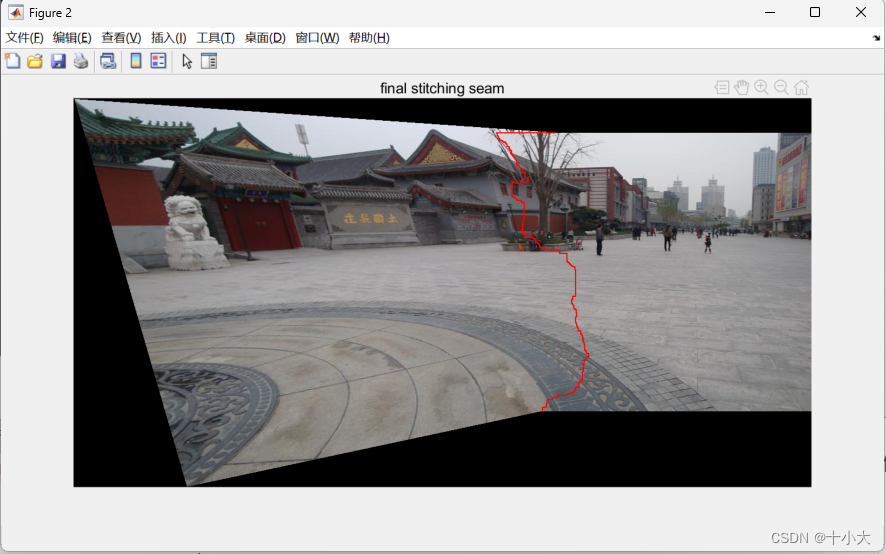
    imgout = gradient_blend(warped_img1, As, warped_img2); 
    
    % 在全尺寸拼接结果中显示缝合线
    SE_seam = strel('square', 3);
    As_seam_ = imdilate(As, SE_seam);
    Bs_seam_ = imdilate(Bs, SE_seam);
    Cs_seam_ = As_seam_ & Bs_seam_;
    imgseam = imgout.*cat(3,(A|B)-Cs_seam_,(A|B)-Cs_seam_,(A|B)-Cs_seam_) + cat(3,Cs_seam_,zeros(sz1,sz2),zeros(sz1,sz2));
    
    figure,imshow(imgseam);
    title('final stitching seam');

至此，本文的代码已解读完毕。

3. 总结思考，试图创新

论文贡献：

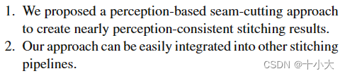
• 提出一个基本感知的接缝拼接方法，几乎和人类预想的拼接缝一致。
• 该方法可以集成到任何拼接方法流中。

也就是说，如果基于接缝的拼接方法没有创新了，那么就考虑排列组合，将最好的接缝融合方法放到你的拼接算法流程中，作为一个创新点。

算法流程回顾：

输入：重叠区域P和翘曲后的两张图像
输出：拼接结果

1. 用欧式准则计算两张输入图像的差异（颜色差异）。
2. 用Ostu算法计算tou。
3. 用sigmoid计算两张输入图像的差异（颜色差异），并根据公式（6）得到平滑项。
4. 用显著性检测方法计算重叠区域的平均像素显著性，并根据公式（8）计算显著性权重。
5. 根据公式（2）计算数据项。（根据代码顺序这一步应该在前面，不过先算谁都无所谓）
6. 图割算法最小化能量还能输，然后梯度融合得到结果。

本文创新思路梳理：在整个图像拼接工作流中，创新图像融合步骤，即基于接缝线的融合方法，改进能量函数（因为能量函数的定义是影响效果最大的）。将最传统的图割算法需要的数据项和平滑项改进，其中平滑项由欧式距离损失改成sigmoid损失，并引入显著性目标检测，得到显著性权重。

直观地，就是将上面的初始能量函数公式变成下面的改进后的公式。

传统能量函数得到的结果：

树枝处放大：

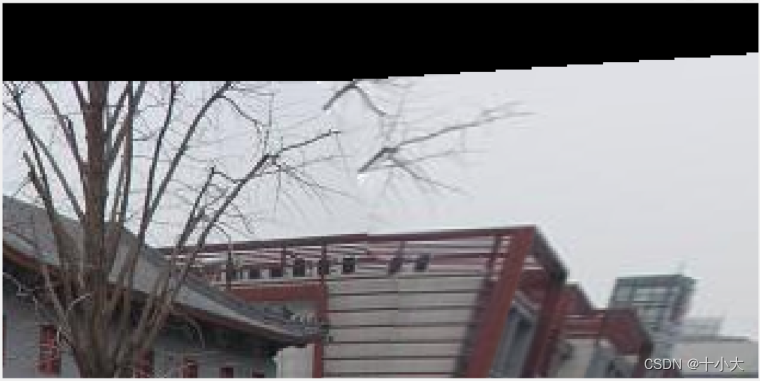
基于感知的能量函数得到的结果：


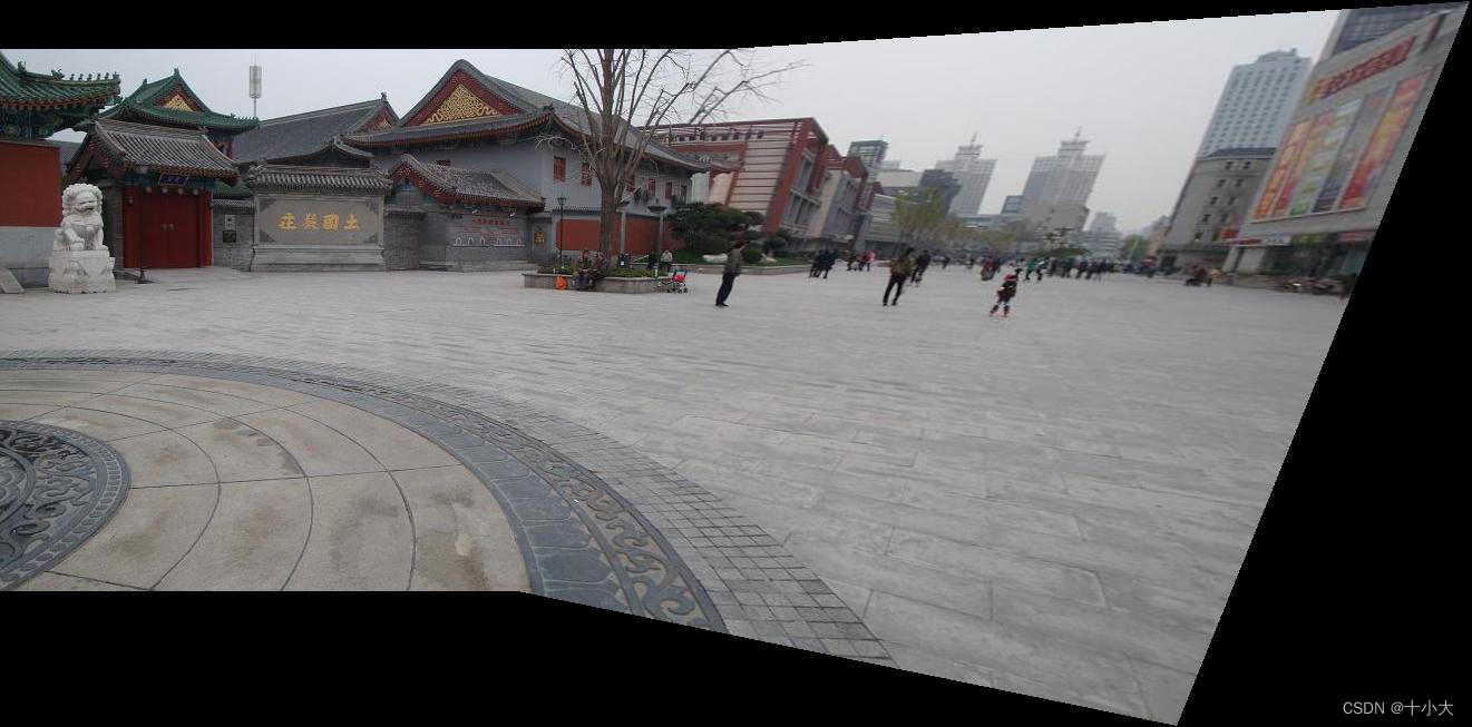
可以看到，初始的能量函数破坏了树枝处原有的结构，而基于感知的能量函数可以淡化这种结构破坏。

另一个有显著结构的例子：

左侧是没有感知的接缝融合结果，右侧是基于感知的接缝融合。很明显，基于感知的效果好，没有破坏线结构，对齐更准。

本文方法应该是目前基于接缝的融合方法中效果最好的了。因为它加入了感知，在重叠区域，接缝可以避免破坏一些显著结构，从而视觉效果很好。