【AI】DETR模型可视化操作

Detr作为目标检测的算法，不同于之前算法的就是注意力机制，注意力机制能够直观看出来模型对图像关注的点，这个直观到底怎么直观呢，我们只听别人说肯定是不行的，上手测试才是最好的方式，像论文中插图那样的使用热度图的方式来展现注意力关注的重点才能叫做直观。幸运的是，官方hands_on手册中给了模型可视化的方式，我也搬过来用一下，方便后续查看。如果有其他模型可视化的操作，也可以借鉴这些代码。

代码是接着上一篇文章的推理模块来的，如果需要运行测试，请先运行上面的代码。

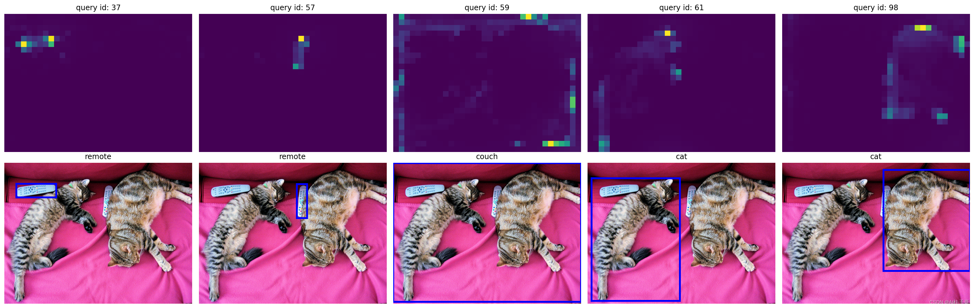
1.可视化编解码多头注意力权重（encoder-decoder multi-head attention weights）

获取权重参数：

# use lists to store the outputs via up-values
conv_features, enc_attn_weights, dec_attn_weights = [], [], []

hooks = [
    model.backbone[-2].register_forward_hook(
        lambda self, input, output: conv_features.append(output)
    ),
    model.transformer.encoder.layers[-1].self_attn.register_forward_hook(
        lambda self, input, output: enc_attn_weights.append(output[1])
    ),
    model.transformer.decoder.layers[-1].multihead_attn.register_forward_hook(
        lambda self, input, output: dec_attn_weights.append(output[1])
    ),
]

# propagate through the model
outputs = model(img)

for hook in hooks:
    hook.remove()

# don't need the list anymore
conv_features = conv_features[0]
enc_attn_weights = enc_attn_weights[0]
dec_attn_weights = dec_attn_weights[0]

可视化展示：

# get the feature map shape
h, w = conv_features['0'].tensors.shape[-2:]

fig, axs = plt.subplots(ncols=len(bboxes_scaled), nrows=2, figsize=(22, 7))
colors = COLORS * 100
for idx, ax_i, (xmin, ymin, xmax, ymax) in zip(keep.nonzero(), axs.T, bboxes_scaled):
    ax = ax_i[0]
    ax.imshow(dec_attn_weights[0, idx].view(h, w))
    ax.axis('off')
    ax.set_title(f'query id: {idx.item()}')
    ax = ax_i[1]
    ax.imshow(im)
    ax.add_patch(plt.Rectangle((xmin, ymin), xmax - xmin, ymax - ymin,
                               fill=False, color='blue', linewidth=3))
    ax.axis('off')
    ax.set_title(CLASSES[probas[idx].argmax()])
fig.tight_layout()

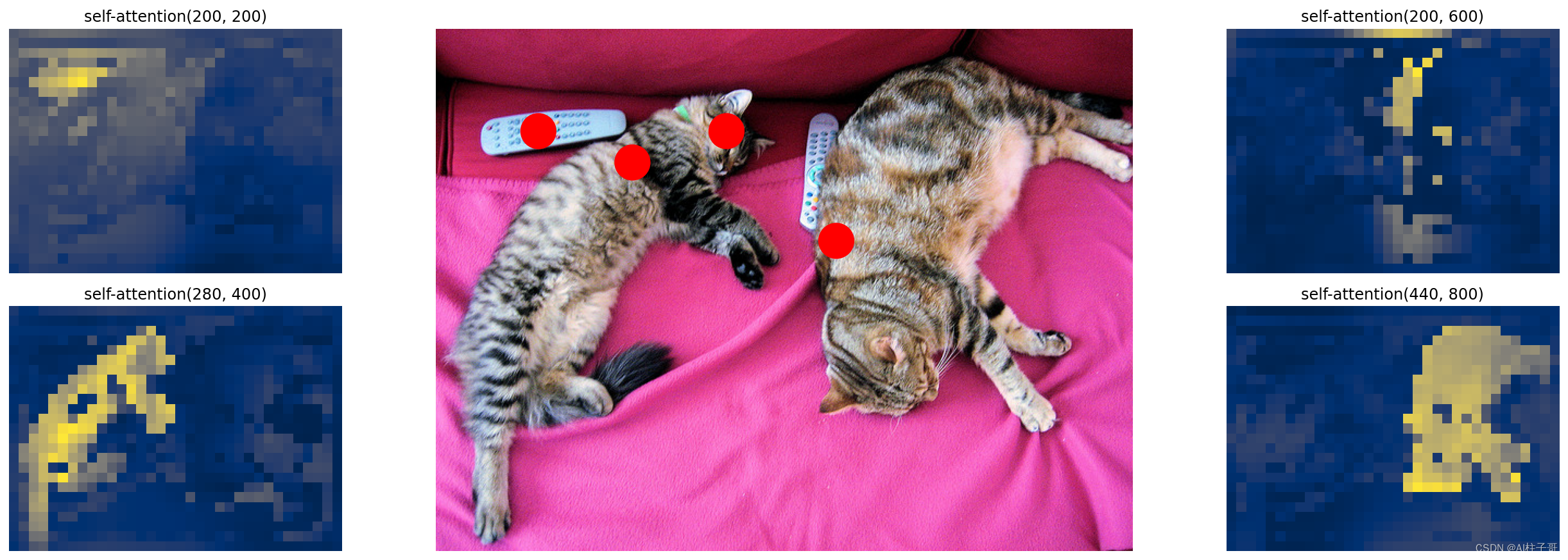
2.可视化编码自注意力权重（encoder self-attention weights）

查看编码权重shape

# output of the CNN
f_map = conv_features['0']
print("Encoder attention:      ", enc_attn_weights[0].shape)
print("Feature map:            ", f_map.tensors.shape)

# output results
# Encoder attention:       torch.Size([850, 850])
# Feature map:             torch.Size([1, 2048, 25, 34])

转换权重矩阵
[H * W, H * W] -> [H,W,H,W]

# get the HxW shape of the feature maps of the CNN
shape = f_map.tensors.shape[-2:]
# and reshape the self-attention to a more interpretable shape
sattn = enc_attn_weights[0].reshape(shape + shape)
print("Reshaped self-attention:", sattn.shape)

查看部分点位

# downsampling factor for the CNN, is 32 for DETR and 16 for DETR DC5
fact = 32

# let's select 4 reference points for visualization
idxs = [(200, 200), (280, 400), (200, 600), (440, 800),]

# here we create the canvas
fig = plt.figure(constrained_layout=True, figsize=(25 * 0.7, 8.5 * 0.7))
# and we add one plot per reference point
gs = fig.add_gridspec(2, 4)
axs = [
    fig.add_subplot(gs[0, 0]),
    fig.add_subplot(gs[1, 0]),
    fig.add_subplot(gs[0, -1]),
    fig.add_subplot(gs[1, -1]),
]

# for each one of the reference points, let's plot the self-attention
# for that point
for idx_o, ax in zip(idxs, axs):
    idx = (idx_o[0] // fact, idx_o[1] // fact)
    ax.imshow(sattn[..., idx[0], idx[1]], cmap='cividis', interpolation='nearest')
    ax.axis('off')
    ax.set_title(f'self-attention{idx_o}')

# and now let's add the central image, with the reference points as red circles
fcenter_ax = fig.add_subplot(gs[:, 1:-1])
fcenter_ax.imshow(im)
for (y, x) in idxs:
    scale = im.height / img.shape[-2]
    x = ((x // fact) + 0.5) * fact
    y = ((y // fact) + 0.5) * fact
    fcenter_ax.add_patch(plt.Circle((x * scale, y * scale), fact // 2, color='r'))
    fcenter_ax.axis('off')