【手搓深度学习算法】用逻辑回归分类双月牙数据集-非线性数据篇

用逻辑回归分类-非线性数据篇

前言

逻辑斯蒂回归是一种广泛使用的分类方法，它是基于条件概率密度函数的最大似然估计的。它的主要思想是将输入空间划分为多个子空间，每个子空间对应一个类别。在每个子空间内部，我们假设输入变量的取值与类别标签的概率成正比。

在逻辑斯蒂回归中，我们首先通过数据进行线性回归，得到的结果再通过sigmoid函数转化为概率，这样就可以得到每个类别的概率。然后，我们可以通过设置一个阈值，如果概率大于阈值，我们就认为这个样本属于这个类别，否则就属于其他类别。这就是逻辑斯蒂回归的基本原理。

逻辑斯蒂回归在现实生活中有很多应用，比如垃圾邮件分类、疾病诊断等。它可以处理非线性关系，而且它的预测结果是概率，这对于处理分类问题非常有用。

在深度学习中，逻辑斯蒂回归的作用主要体现在两个方面：一是作为一种基础的分类方法，它可以用于二分类问题，比如判断一个邮件是否为垃圾邮件；二是作为一种特征提取方法，它可以用于提取输入数据的特征，这些特征可以被其他深度学习模型使用。

本文重点总结逻辑斯蒂回归在非线性数据集上的应用方法，对线性数据分类还有疑惑的跳转
逻辑斯蒂回归多分类-线性数据篇

名词解释

回归

很多初学（复习）统计学或者深度学习算法的同学（包括我），对“回归”这个名词可能感觉有点疑惑，因为它既熟悉又陌生，熟悉是因为它在现实生活中也很常见，比如香港回归，澳门回归。。。，陌生的是当它跟统计学名词联系在一起，又会让人有点摸不着头脑，什么线性回归，逻辑斯蒂回归。。。，为此，我专门查找了相关资料，总结如下：

在统计学和深度学习中，“回归”这个术语的含义主要是关于预测一个连续的目标变量。这个目标变量可以是任何可以连续变化的东西，比如销售额、房价、股票价格等。在这种情况下，“回归”的意思是“倒推”或者“预测”。

在统计学中，我们使用回归分析来研究一个或多个自变量（即影响因素）与一个因变量（即我们想要预测的结果）之间的关系。例如，我们可能会使用回归分析来研究房价与房屋面积、位置、年份等因素的关系。在这种情况下，我们的目标是找到一个函数，这个函数可以根据这些因素预测房价。这就是“回归”的含义：我们是在“倒推”或者“预测”房价。

在深度学习中，我们也使用回归模型，但是这里的“回归”更多的是指预测一个连续的目标变量。例如，我们可能会使用深度学习的回归模型来预测一个物品的评分，或者预测一个人的年龄。在这种情况下，我们的目标是找到一个函数，这个函数可以根据一些输入特征预测这个连续的目标变量。这也是“回归”的含义：我们是在“倒推”或者“预测”这个连续的目标变量。

总的来说，无论是在统计学还是在深度学习中，“回归”的含义都是“倒推”或者“预测”一个连续的目标变量。这个目标变量可以是任何可以连续变化的东西，比如销售额、房价、股票价格、评分、年龄等。我们的目标是找到一个函数，这个函数可以根据一些输入特征预测这个连续的目标变量。

使用逻辑斯蒂回归对线性数据和非线性数据进行训练和预测有什么异同

逻辑斯蒂回归是一种广义的线性模型，可以用于二分类问题。它本质上是线性回归模型，但在输出层使用了sigmoid函数，将线性回归的输出映射到(0,1)区间，表示概率。

在处理线性数据时，逻辑斯蒂回归的表现与普通线性回归类似。训练过程主要是通过最小化预测概率与实际标签之间的损失函数来进行的。在预测阶段，给定新的输入数据，模型会输出每个类别的概率。

然而，当处理非线性数据时，逻辑斯蒂回归仍然保持其线性特性。这并不意味着它不能处理非线性问题，而是说它通过引入非线性映射函数（如sigmoid函数）来处理数据内在的非线性关系。这种处理方式允许逻辑斯蒂回归在非线性数据上表现出色，而无需改变其作为线性回归模型的内在机制。

总结来说，逻辑斯蒂回归在处理非线性数据时，其训练和预测过程与处理线性数据时的主要区别在于如何解释和使用模型的输出。在任何情况下，它都保持了其作为线性模型的特性，只是在更高层次上（即通过sigmoid函数）引入了非线性。

虽然逻辑回归本质可以处理非线性数据，但它本质上还是一个线性模型，很多情况下对非线性数据不能很好的拟合，我们可以运用特征工程对输入数据集进行处理，本文通过引入多项式变换进行试验，比较引入前后的准确率和决策边界。

对输入数据进行多项式变换在逻辑斯蒂回归中主要有两个作用：

• 处理非线性问题：当数据内在存在非线性关系时，通过多项式变换可以将这些非线性关系转换为线性关系，使得逻辑斯蒂回归能够更好地拟合数据。
• 增加模型的灵活性：多项式变换允许模型捕捉到更复杂的输入和输出之间的关系，从而提高了模型的预测能力。 *

实现

工具函数

Sigmoid

Sigmoid函数是一种常用的激活函数，它将任意实数映射到0和1之间。Sigmoid函数的定义如下：

$$\sigma (x)=\frac{1}{1+e^{?x}}$$

其中，$x$是输入，$\sigma (x)$是输出。

Sigmoid函数的图像如下(不平滑因为是我自己生成的。。。)：

Sigmoid函数的主要特性包括：

1. 单调递增：对于所有的$x$，$\sigma (x)$都是单调递增的。

2. 输出范围在0和1之间：对于所有的$x$，$0\le \sigma (x)\le 1$。

3. 可微：Sigmoid函数是可微的，这使得它可以用于神经网络的反向传播算法。

def sigmoid(data):
    return 1 / (1+np.exp(-data))

数据预处理函数

对数据进行标准化和多项式变换，本文将分别比较“不使用多项式变换”、“不同角度的多项式变换”对准确率和拟合、泛化的影响

def prepare_data(data, normalize_data=False, polynomial_transform_degree=-1): 
  assert isinstance(data, np.ndarray), "Data must be a numpy array" 

  # 标准化特征矩阵  
  if normalize_data:  
      features_mean = np.mean(data, axis=0)  #特征的平均值
      features_dev = np.std(data, axis=0)    #特征的标准偏差
      features = (data - features_mean) / features_dev  #标准化数据
  else:  
      features_mean = None  
      features_dev = None  
      features = data

  # 多项式特征变换
  if (polynomial_transform_degree != -1):
      degree = polynomial_transform_degree
      new_features = []
      for i in range(degree + 1):
          new_features.append(np.power(features, i))
      features = np.column_stack(new_features)

  data_processed = features
  # 返回处理后的数据
  return data_processed, features_mean, features_dev

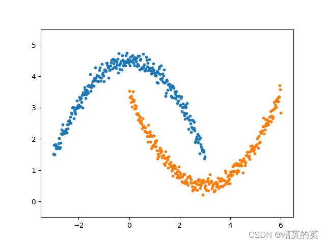
非线性数据模拟生成函数

定义了一个名为moon2Data的函数，用于生成模拟数据，这些数据类似于月亮的形状

函数名为moon2Data，它接受两个参数：datanum和show。datanum表示要生成的点的数量，show是一个布尔值，决定是否显示生成的点。函数的返回类型是np.ndarray，即NumPy数组。

生成月亮形状的第一部分（代表类0的数据）。

x1 = np.linspace(-3, 3, datanum)
noise = np.random.randn(datanum) * 0.15
y1 = -np.square(x1) / 3 + 4.5 + noise

x1是在-3到3之间的均匀分布的datanum`个值。然后添加了高斯噪声。对于y1，它是x1的负平方除以3再加4.5后再加上噪声。

这部分代码将x1和y1重新整形为列向量，并添加一个全为0的列，用于代表分类标签（这里使用0表示类0）。

class0 = np.concatenate((x1.reshape(datanum,1), y1.reshape(datanum,1), np.zeros((datanum, 1))), axis=1)

生成月亮形状的第二部分（代表类1的数据）。

x2 = np.linspace(0, 6, datanum)
noise = np.random.randn(datanum) * 0.15
y2 = np.square(x2 - 3) / 3 + 0.5 + noise

x2是在0到6之间的均匀分布的datanum`个值。然后添加了高斯噪声。对于y2，它是x2减去3后的平方除以3再加0.5后再加上噪声。
与生成类0的数据类似，但是添加了一个全为1的列作为分类标签。

class1 = np.concatenate((x2.reshape(datanum,1), y2.reshape(datanum,1), np.ones((datanum, 1))), axis=1)

将类0和类1的数据合并为一个大的NumPy数组。

ret = np.concatenate((class0, class1), axis=0)

如果show参数为True，则使用matplotlib显示生成的点。这主要用于可视化目的。

if (show):
    plt.clf()  # 清除当前图形
    plt.axis([-3.5, 6.5, -.5, 5.5])  # 设置轴的范围
    plt.scatter(x1, y1, s=10)  # 绘制类0的点
    plt.scatter(x2, y2, s=10)  # 绘制类1的点
    plt.draw()  # 更新图形显示
    plt.pause(.1)  # 暂停0.1秒，以便查看图形
    plt.show()  # 显示图形

最后，函数返回合并后的数据。

return ret

def moon2Data(datanum, show = False) -> np.ndarray:
    x1 = np.linspace(-3, 3, datanum)
    noise = np.random.randn(datanum) * 0.15
    y1 = -np.square(x1) / 3 + 4.5 + noise
    class0 = np.concatenate((x1.reshape(datanum,1), y1.reshape(datanum,1), np.zeros((datanum, 1))), axis=1)
    x2 = np.linspace(0, 6, datanum)
    noise = np.random.randn(datanum) * 0.15
    y2 = np.square(x2 - 3) / 3 + 0.5 + noise
    class1 = np.concatenate((x2.reshape(datanum,1), y2.reshape(datanum,1), np.ones((datanum, 1))), axis=1)
    ret = np.concatenate((class0, class1), axis=0)
    if (show):
        plt.clf()
        plt.axis([-3.5, 6.5, -.5, 5.5])
        plt.scatter(x1, y1, s=10)
        plt.scatter(x2, y2, s=10)
        plt.draw()
        plt.pause(.1)
        plt.show()
    return ret

逻辑斯蒂回归类

以下代码在名为"LogisticRegression"的类中，大部分代码都和线性篇里面介绍的相同

初始化

将传入的数据集和标签记录下来以便进一步处理，同时初始化权重矩阵

def __init__(self, data,labels, normalize = False, polynomial_transform_degree = -1) -> None:
        self.normalize = normalize
        self.polynomial_transform_degree = polynomial_transform_degree
        data_processed, mean, dev = prepare_data(data, normalize, polynomial_transform_degree)
        self.data = data_processed
        self.labels = labels
        self.unique_labels = np.unique(labels) #取标签中的类的名称的集合
        self.num_examples = self.data.shape[0] #取数据集中样本的数量
        self.num_features = self.data.shape[1] #取数据集中的特征个数
        num_unique_labels = self.unique_labels.shape[0] #取标签中类的个数
        self.theta = np.zeros((num_unique_labels,self.num_features)) #初始化权重向量，因为我们是多分类，所以权重是 “分类数量 x 特征个数”的矩阵

训练函数

对每个可能的分类执行训练过程，因为逻辑斯蒂回归通常用于处理二分类问题，所以每次都将当前分类的标签置为“1”，其他分类的标签置为“0”

def train(self, lr = 0.01, max_iter = 1000):
    cost_histories = [] #记录损失历史记录，以便可视化
    for label_index, unique_label in enumerate(self.unique_labels): #对所有可能的分类进行遍历
        current_initial_theta = np.copy(self.theta[label_index].reshape(self.num_features, 1)) #复制对应的权重向量，以避免直接修改
        current_labels = (self.labels == unique_label).astype(float) #等于当前标签的置为1，否则为0
        (current_theta, cost_history) = LogisticRegression.gradient_descent(self.data, current_labels, current_initial_theta, max_iter) #执行梯度下降过程
        self.theta[label_index] = current_theta.T #记录当前分类最终的权重向量
        cost_histories.append(cost_history) #记录当前分类最终的损失历史记录
    return cost_histories, self.theta

梯度下降过程

在规定的迭代次数里执行梯度下降，每次权重向量都减去学习率乘以当前梯度，通过迭代优化模型的参数（也就是权重向量 $\theta$），使得模型的预测结果与真实标签之间的差异（也就是损失函数）最小。

gradient_descent 方法的主要任务是执行梯度下降的迭代过程。它接收五个参数：数据集 data、标签 labels、当前的初始权重向量 current_initial_theta、学习率 lr 和最大迭代次数 max_iter。在每次迭代中，它会调用 gradient_step 方法计算梯度，然后根据梯度更新权重向量。同时，它还会记录每次迭代后的损失值，以便于后续的可视化或者调试。

gradient_step 方法的主要任务是计算梯度。它接收三个参数：数据集 data、标签 labels 和当前的权重向量 theta。首先，它会计算预测值 predictions，然后计算预测值与真实标签之间的差异 label_diff。最后，它会计算梯度 gradients，并返回梯度的平均值。

在这里，梯度的计算公式为：

$${?}_{\theta }J(\theta )=\frac{1}{N}\sum _{i=1}^N(h_{\theta }(x^{(i)})?y^{(i)})x^{(i)}$$

其中，$N$ 是数据集的大小，$h_{\theta }(x^{(i)})$ 是预测值，$y^{(i)}$ 是真实标签，$x^{(i)}$ 是第 $i$ 个数据点。

这个公式的含义是，对于每一个数据点，我们都计算了预测值与真实标签之间的差异，然后乘以该数据点的特征向量，最后将所有数据点的结果加起来，再除以数据集的大小，得到的就是梯度。

这个梯度反映了模型预测结果与真实标签之间的差异，我们希望通过不断地调整权重向量，使得这个差异越来越小，从而提高模型的预测效果。

def gradient_descent(data, labels, current_initial_theta, lr, max_iter):
    cost_history = [] #损失历史
    num_features = data.shape[1] #特征数量
    optimized_theta = current_initial_theta #取初始权重
    for _ in range(max_iter): #在规定的迭代次数范围内迭代
        optimized_theta -= float(lr) * LogisticRegression.gradient_step(data, labels, optimized_theta).reshape(num_features, 1) #执行单步更新权重
        cost_history.append(LogisticRegression.cost_function(data, labels, optimized_theta)) # 记录损失历史
    optimized_theta = optimized_theta.reshape(num_features, 1)
    return optimized_theta, cost_history

def gradient_step(data, labels, theta):
    num_examples = labels.shape[0] #样本数量
    predictions = LogisticRegression.predict(data.T, theta) #特征和权重的点积然后执行sigmoid，得到概率
    label_diff = predictions - labels #差异
    gradients = (1/num_examples)*np.dot(data.T, label_diff) #计算梯度，差异和数据的点积除以样本数量
    return gradients.T.flatten() #将梯度转换为一维

损失函数

主要功能是计算模型的预测结果与真实标签之间的差异，也就是损失函数。

cost_function 方法的主要任务是计算损失函数。它接收三个参数：数据集 data、标签 labels 和当前的权重向量 theta。
首先，它会计算预测值 prediction，
然后根据预测值和真实标签的关系，计算两部分的损失 y_is_set_cost 和 y_is_not_set_cost。
最后，它会将这两部分的损失相加，然后除以数据集的大小，得到的就是损失函数。

在这里，损失函数的计算公式为：

$$J(\theta )=?\frac{1}{N}\left[\sum _{i=1}^N{y}^{(i)}\log (h_{\theta }(x^{(i)}))+(1?y^{(i)})\log (1?h_{\theta }(x^{(i)}))\right]$$

其中，$N$ 是数据集的大小，$y^{(i)}$ 是第 $i$ 个数据点的真实标签，$h_{\theta }(x^{(i)})$ 是第 $i$ 个数据点的预测值。

这个公式的含义是，对于每一个数据点，如果它的真实标签是1，那么我们就计算 $\log (h_{\theta }(x^{(i)}))$ 的值；如果它的真实标签是0，因为$h_{\theta }(x^{(i)})$ 计算的是$predict=1$的概率，所以我们就计算 $\log (1?h_{\theta }(x^{(i)}))$ 的值。然后，我们将所有数据点的结果加起来，再除以数据集的大小，得到的就是损失函数。

损失函数反映了模型预测结果与真实标签之间的差异，我们希望通过不断地调整权重向量，使得这个差异越来越小，从而提高模型的预测效果。

def cost_function(data, labels, theta):
    num_examples = data.shape[0] #样本数量
    prediction = LogisticRegression.predict(data.T, theta) #特征和权重的点积然后执行sigmoid，得到概率
    y_is_set_cost = np.dot(labels[labels == 1].T, np.log(prediction[labels == 1])) #当标签等于1时的权重向量
    y_is_not_set_cost = np.dot(1-labels[labels == 0].T, np.log(1-prediction[labels == 0])) #当标签等于0时的权重向量
    cost = (-1/num_examples) * (y_is_set_cost+y_is_not_set_cost) # 计算整体损失
    return cost
    

预测计算函数

特征和权重的点积然后计算Sigmoid得到概率

def predict(data, theta):
        predictions = sigmoid(np.dot(data.T, theta))
        return predictions

验证计算函数

验证计算函数先对输入特征矩阵进行预测计算，然后对每个样本，计算其概率最大值，最后将每个样本的最佳预测分类和每个样本属于三个分类的概率返回。

def predict_test(self, data):
    num_examples = data.shape[0] #样本数量
    prob = LogisticRegression.predict(data.T, self.theta.T) #计算预测值
    max_prob_index = np.argmax(prob, axis = 1) #最大的概率值的index
    class_prediction = np.empty(max_prob_index.shape, dtype=object) # 初始化预测结果
    for index,label in enumerate(self.unique_labels):
        class_prediction[max_prob_index == index] = label # 取预测值
    return class_prediction.reshape((num_examples,1)), prob

完整流程

1. 数据集的准备和分割:

   • 首先调用 moon2Data 函数生成一个非线性可分的数据集
   • 数据集被随机打乱，然后分为训练集和测试集，比例为 80% 训练数据和 20% 测试数据。

2. 逻辑回归模型的初始化:

   • 创建 LogisticRegression 类的实例 logistic_reg，传入训练数据、训练标签，并设置数据标准化和多项式特征转换的参数。这些步骤对数据进行预处理，以提高模型的性能。

3. 模型训练:

   • 调用 logistic_reg 实例的 train 方法，传入学习率和最大迭代次数，开始训练过程。训练过程中，模型的参数（权重）会通过梯度下降算法进行优化，以最小化损失函数。

4. 损失历史的可视化:

   • 使用 matplotlib 库绘制损失历史曲线，这有助于观察模型在训练过程中损失的变化情况。

5. 模型测试和预测信息的显示:

   • 使用训练好的模型对测试数据进行预测，并调用 show_predict_info 函数显示预测的准确率和错误预测的详细信息。

6. 测试数据的可视化:

   • 根据测试数据的标签将数据分为两类，并使用散点图进行可视化，以展示数据的分布情况。

7. 非线性决策边界的绘制:

   • 生成一个网格，覆盖当前图形的 x 和 y 轴范围。
   • 使用训练好的模型对这个网格上的每个点进行预测，以确定它们属于哪个类别。
   • 绘制等高线（决策边界），这有助于直观地理解模型是如何将不同类别的数据分开的。

8. 结束:

   • 最后，再次使用训练数据进行预测，并显示预测信息，这有助于评估模型在训练集上的性能。

通过逻辑回归模型对数据进行分类，并通过可视化来评估模型的性能。

import pandas as pd
import matplotlib.pyplot as plt
def main():
    moon_shape_dataset = moon2Data(300)
    print (moon_shape_dataset.shape)
    np.random.shuffle(moon_shape_dataset)
    train_dataset = moon_shape_dataset[:int(len(moon_shape_dataset)*0.8):]
    test_dataset = moon_shape_dataset[int(len(moon_shape_dataset)*0.8):]
    train_labels = train_dataset[:,-1:]
    test_labels = test_dataset[:,-1:]
    train_data = train_dataset[:,:-1]
    test_data = test_dataset[:,:-1]
    logistic_reg = LogisticRegression(train_data, train_labels, normalize=True, polynomial_transform_degree=3)
    loss_history, theta = logistic_reg.train(0.001, 50000)
    plt.close()
    plt.plot(loss_history[0])
    plt.plot(loss_history[1])
    plt.show()
    
    prediction, prop = logistic_reg.predict_test(test_data)
    show_predict_info(prediction, prop, test_labels)
    
    class0_data = test_dataset[test_dataset[:,-1]==0.0]
    class1_data = test_dataset[test_dataset[:,-1]==1.0]
    
    plt.close()
    plt.scatter(class0_data[:,0], class0_data[:,1])
    plt.scatter(class1_data[:,0], class1_data[:,1]) 
 
    
    # 绘制非线性决策边界  
    x_min, x_max = plt.xlim()  
    y_min, y_max = plt.ylim()  
    x_grid = np.linspace(x_min, x_max, 100)
    y_grid = np.linspace(y_min, y_max, 100)

    x,y = np.meshgrid(x_grid, y_grid)
    grid = np.concatenate((x.reshape(-1,1), y.reshape(-1,1)), axis=1)

    values, probs = logistic_reg.predict_test(grid)
    values = values.reshape(100,100).astype("float")
    # 绘制等高线
    plt.contour(x, y, values)
    # 添加标题和轴标签
    plt.title('Non Linear Plot')
    plt.xlabel('X position')
    plt.ylabel('Y position')
    # 显示图形
    plt.show()
    prediction, prop = logistic_reg.predict_test(train_data)
    show_predict_info(prediction, prop, train_labels)
    
    
if (__name__ == "__main__"):
    main()
    

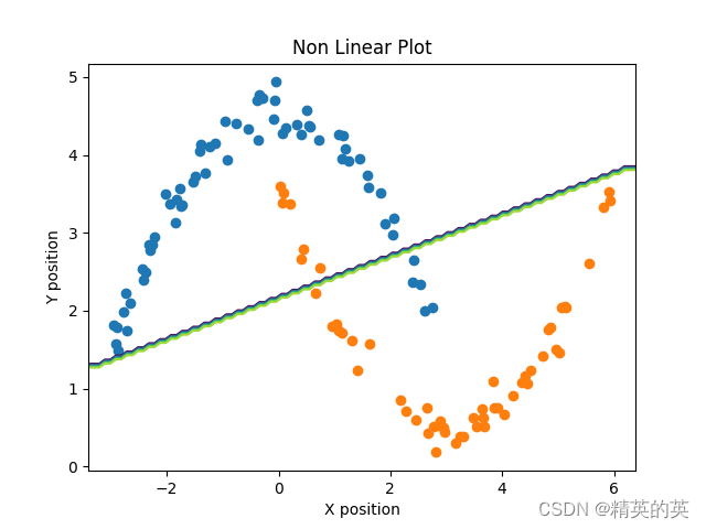
不使用多项式变换时的准确率和决策边界

我们通过传入“-1”告诉数据处理函数不进行多项式变换

    logistic_reg = LogisticRegression(train_data, train_labels,
     normalize=True, 
     polynomial_transform_degree=-1)

可以看到虽然准确率还不错“Accuracy is [0.9]”，但是决策边界明显还是线性的，在训练集和测试集都没有做到拟合

使用多项式设置degree=2时的准确率和决策边界

我们通过传入“2”告诉数据处理函数进行多项式变换

    logistic_reg = LogisticRegression(train_data, train_labels,
     normalize=True, 
     polynomial_transform_degree=2)

可以看到准确率和上面几乎相同，而且决策边界也没有拟合数据，这是因为：
当degree=2时，多项式变换会在原始特征的基础上添加它们的平方项和所有可能的两两特征组合（交互项）。这确实增加了模型的非线性能力，但是否足以捕捉到数据的非线性关系，以及决策边界的形状，取决于几个因素：

1. 数据集的特征数：如果原始数据集只有一个特征，那么即使是二次多项式变换，也只会产生一个平方项，这在二维空间中仍然是一条抛物线，而不是复杂的非线性边界。如果有两个或更多的特征，二次多项式变换会产生交互项，这可能会导致非线性决策边界，但这仍然取决于数据的分布。

2. 数据的分布：如果数据的真实分布是高度非线性的，那么即使添加了平方项和交互项，二次多项式变换可能仍然不足以捕捉到所有的非线性关系。在这种情况下，决策边界可能仍然看起来相对平滑和简单。

3. 模型的限制：逻辑斯蒂回归是一个线性模型，它的决策边界是特征空间中的一个超平面。即使通过多项式变换增加了特征，逻辑斯蒂回归仍然试图找到一个超平面来分隔这些特征。
   

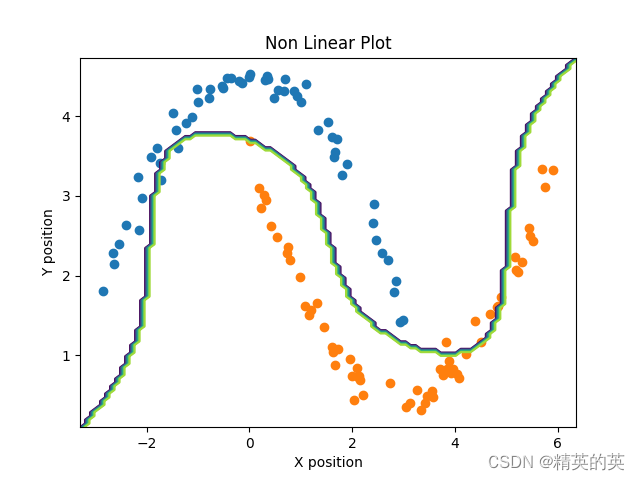
使用多项式设置degree=5时的准确率和决策边界

我们通过传入“5”告诉数据处理函数进行多项式变换

    logistic_reg = LogisticRegression(train_data, train_labels,
     normalize=True, 
     polynomial_transform_degree=5)

可以看到在测试数据集上变现除了良好的准确率Accuracy is [0.99166667]，而且决策边界也充分拟合了数据

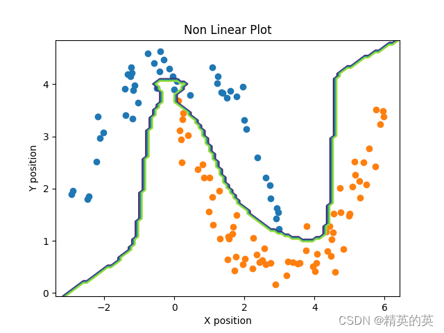
使用多项式设置degree=15时的准确率和决策边界

我们通过传入“15”告诉数据处理函数进行多项式变换

    logistic_reg = LogisticRegression(train_data, train_labels,
     normalize=True, 
     polynomial_transform_degree=15)

可以看到测试集准确率为Accuracy is [0.95833333]，已经出现了过拟合（虽然不明显，可见逻辑斯蒂回归还是很强大的…）

完整代码（数据集自动生成，不用下载）

import numpy as np    
from scipy.optimize import minimize
from 生成非线性数据集 import moon2Data
from sklearn.preprocessing import PolynomialFeatures

def sigmoid(data):
    return 1 / (1+np.exp(-data))

def prepare_data(data, normalize_data=False, polynomial_transform_degree=-1): 
  assert isinstance(data, np.ndarray), "Data must be a numpy array" 

  # 标准化特征矩阵  
  if normalize_data:  
      features_mean = np.mean(data, axis=0)  #特征的平均值
      features_dev = np.std(data, axis=0)    #特征的标准偏差
      features = (data - features_mean) / features_dev  #标准化数据
  else:  
      features_mean = None  
      features_dev = None  
      features = data

  # 多项式特征变换
  if (polynomial_transform_degree != -1):
      degree = polynomial_transform_degree
      new_features = []
      for i in range(degree + 1):
          new_features.append(np.power(features, i))
      features = np.column_stack(new_features)

  data_processed = features
  # 返回处理后的数据
  return data_processed, features_mean, features_dev

def show_predict_info(prediction, prop, labels):
    accuracy = sum(prediction == labels) / len(labels)
    print("Accuracy is {}".format(accuracy))
    fail_predict = []
    for index, item in enumerate(prediction.flatten()):
        if (item != labels.flatten()[index]):
            info = {}
            info["index"]=index
            info["predict"]=item
            info["actual"]=labels.flatten()[index]
            fail_predict.append(info)
    for predict_info in fail_predict:
        print("Predict is {} prop is {}, actual is {} prop is {}".format(
            predict_info["predict"], prop[predict_info["index"], [int(predict_info["predict"])]],
            predict_info["actual"], prop[predict_info["index"], [int(predict_info["actual"])]]))

class LogisticRegression:
    '''
    1. 对数据进行预处理操作
    2. 先得到所有的特征个数
    3. 初始化参数矩阵
    '''
    def __init__(self, data,labels, normalize = False, polynomial_transform_degree = -1) -> None:
        self.normalize = normalize
        self.polynomial_transform_degree = polynomial_transform_degree
        data_processed, mean, dev = prepare_data(data, normalize, polynomial_transform_degree)
        self.data = data_processed
        self.labels = labels
        self.unique_labels = np.unique(labels) #取标签中的类的名称的集合
        self.num_examples = self.data.shape[0] #取数据集中样本的数量
        self.num_features = self.data.shape[1] #取数据集中的特征个数
        num_unique_labels = self.unique_labels.shape[0] #取标签中类的个数
        self.theta = np.zeros((num_unique_labels,self.num_features)) #初始化权重向量，因为我们是多分类，所以权重是 “分类数量 x 特征个数”的矩阵
        
    def train(self, lr = 0.01, max_iter = 1000):
        cost_histories = [] #记录损失历史记录，以便可视化
        for label_index, unique_label in enumerate(self.unique_labels): #对所有可能的分类进行遍历
            current_initial_theta = np.copy(self.theta[label_index].reshape(self.num_features, 1)) #复制对应的权重向量，以避免直接修改
            current_labels = (self.labels == unique_label).astype(float) #等于当前标签的置为1，否则为0
            (current_theta, cost_history) = LogisticRegression.gradient_descent(self.data, current_labels, current_initial_theta, max_iter) #执行梯度下降过程
            #(current_theta, cost_history) = LogisticRegression.gradient_descent(self.data, current_labels, current_initial_theta, '''lr,''' max_iter) #执行梯度下降过程
            self.theta[label_index] = current_theta.T #记录当前分类最终的权重向量
            cost_histories.append(cost_history) #记录当前分类最终的损失历史记录
        return cost_histories, self.theta
        
    
    @staticmethod
    def gradient_descent(data, labels, current_initial_theta, max_iter):
        cost_history = []
        num_features = data.shape[1]
        #scipy.optimize.minimize`函数被用于实现梯度下降算法。这个函数的主要作用是找到一个最小值点，使得目标函数的值最小。
        result = minimize(
            #要优化的目标
            fun = lambda current_theta:LogisticRegression.cost_function(data, labels, current_theta.reshape(num_features, 1)),
            #初始化的权重参数
            x0 = current_initial_theta.flatten(),
            #选择优化策略, 表示使用共轭梯度法进行优化
            method='CG',
            #梯度下降迭代计算公式
            jac= lambda current_theta:LogisticRegression.gradient_step(data, labels,current_theta.reshape(num_features, 1)),
            #记录结果
            callback = lambda current_theta:cost_history.append(LogisticRegression.cost_function(data, labels, current_theta.reshape(num_features, 1))),
            #迭代次数
            options = {'maxiter':max_iter}
        )
        if not (result.success):
            raise ArithmeticError('Can not minimize cost function ' + result.message)
        #minimize`函数的输出是一个结果对象，其中`result.x`是找到的最小值点，`result.fun`是在最小值点处的目标函数值。
        optimized_theta = result.x.reshape(num_features, 1)
        return optimized_theta, cost_history
    
    '''
    @staticmethod
    def gradient_descent(data, labels, current_initial_theta, lr, max_iter):
        cost_history = [] #损失历史
        num_features = data.shape[1] #特征数量
        optimized_theta = current_initial_theta #取初始权重
        for index, _ in enumerate(range(max_iter)): #在规定的迭代次数范围内迭代
            optimized_theta -= float(lr) * LogisticRegression.gradient_step(data, labels, optimized_theta).reshape(num_features, 1) #执行单步更新权重
            loss = LogisticRegression.cost_function(data, labels, optimized_theta)
            if (index % 10 == 0):
                print("Step {} loss is {}".format(index, loss))
            cost_history.append(loss) # 记录损失历史
        optimized_theta = optimized_theta.reshape(num_features, 1)
        return optimized_theta, cost_history
    '''
    @staticmethod
    def gradient_step(data, labels, theta):
        num_examples = labels.shape[0] #样本数量
        predictions = LogisticRegression.predict(data.T, theta) #特征和权重的点积然后执行sigmoid，得到概率
        label_diff = predictions - labels #差异
        gradients = (1/num_examples)*np.dot(data.T, label_diff) #计算梯度，差异和数据的点积除以样本数量
        return gradients.T.flatten() #将梯度转换为一维
    
    
    @staticmethod
    def cost_function(data, labels, theta):
        num_examples = data.shape[0] #样本数量
        prediction = LogisticRegression.predict(data.T, theta) #特征和权重的点积然后执行sigmoid，得到概率
        y_is_set_cost = np.dot(labels[labels == 1].T, np.log(prediction[labels == 1])) #当标签等于1时的权重向量
        y_is_not_set_cost = np.dot(1-labels[labels == 0].T, np.log(1-prediction[labels == 0])) #当标签等于0时的权重向量
        cost = (-1/num_examples) * (y_is_set_cost+y_is_not_set_cost) # 计算整体损失
        return cost
    
    
    @staticmethod
    def predict(data, theta):
        predictions = sigmoid(np.dot(data.T, theta))
        return predictions
    
    def predict_test(self, data):
        data_processed = prepare_data(data, self.normalize, self.polynomial_transform_degree)[0]
        num_examples = data_processed.shape[0] #样本数量
        prob = LogisticRegression.predict(data_processed.T, self.theta.T) #计算预测值
        max_prob_index = np.argmax(prob, axis = 1) #最大的概率值的index
        class_prediction = np.empty(max_prob_index.shape, dtype=object) # 初始化预测结果
        for index,label in enumerate(self.unique_labels):
            class_prediction[max_prob_index == index] = label # 取预测值
        return class_prediction.reshape((num_examples,1)), prob

import pandas as pd
import matplotlib.pyplot as plt
def main():
    '''iris_dataset = "J:\\MachineLearning\\数据集\\Iris\\iris.data"
    dataset_src = pd.read_csv(iris_dataset).values
    np.random.shuffle(dataset_src)
    print("The shape of original dataset is {}".format(dataset_src.shape))
    train_data = dataset_src[:int(len(dataset_src)*0.8)]
    test_data = dataset_src[int(len(dataset_src)*0.8):]
    train_dataset = train_data[:, :-1].astype('float')
    train_label = train_data[:, -1].reshape(-1,1)
    test_dataset = test_data[:, :-1].astype('float')
    test_label = test_data[:, -1].reshape(-1,1)
    print("The shape of train dataset is {}".format(train_dataset.shape))
    print("The shape of test dataset is {}".format(test_dataset.shape))
    print("The shape of train label is {}".format(train_label.shape))
    print("The shape of test label is {}".format(test_label.shape))
    # 创建一个字典，将每种花的名称映射到一个唯一的整数
    flower_dict = {
       'Iris-versicolor': 0,
       'Iris-setosa': 1,
       'Iris-virginica': 2
    }
    
    # 使用字典来转换数组
    converted_array = [[flower_dict[item[0]]] for item in train_label]
    train_label = np.array(converted_array).reshape(-1,1).astype('int')
    converted_array = [[flower_dict[item[0]]] for item in test_label]
    test_label = np.array(converted_array).reshape(-1,1).astype('int')

    print(train_dataset)
    print(train_label)
    logistic_reg = LogisticRegression(np.array(train_dataset), np.array(train_label))
    (loss_history, theta) = logistic_reg.train(lr=0.001, max_iter= 10000)
    plt.plot(loss_history[0])
    plt.plot(loss_history[1])
    plt.plot(loss_history[2])
    

    prediction, prop = logistic_reg.predict_test(test_dataset)
    show_predict_info(prediction, prop, test_label)
    
    
    prediction, prop = logistic_reg.predict_test(train_dataset)
    show_predict_info(prediction, prop, train_label)
    '''
    moon_shape_dataset = moon2Data(300)
    print (moon_shape_dataset.shape)
    np.random.shuffle(moon_shape_dataset)
    train_dataset = moon_shape_dataset[:int(len(moon_shape_dataset)*0.8):]
    test_dataset = moon_shape_dataset[int(len(moon_shape_dataset)*0.8):]
    train_labels = train_dataset[:,-1:]
    test_labels = test_dataset[:,-1:]
    train_data = train_dataset[:,:-1]
    test_data = test_dataset[:,:-1]
    logistic_reg = LogisticRegression(train_data, train_labels, normalize=True, polynomial_transform_degree=15)
    loss_history, theta = logistic_reg.train(0.001, 50000)
    plt.close()
    plt.plot(loss_history[0])
    plt.plot(loss_history[1])
    plt.show()
    
    prediction, prop = logistic_reg.predict_test(test_data)
    show_predict_info(prediction, prop, test_labels)
    
    class0_data = test_dataset[test_dataset[:,-1]==0.0]
    class1_data = test_dataset[test_dataset[:,-1]==1.0]
    
    plt.close()
    plt.scatter(class0_data[:,0], class0_data[:,1])
    plt.scatter(class1_data[:,0], class1_data[:,1]) 
 
    
    # 绘制非线性决策边界  
    x_min, x_max = plt.xlim()  
    y_min, y_max = plt.ylim()  
    x_grid = np.linspace(x_min, x_max, 100)
    y_grid = np.linspace(y_min, y_max, 100)

    x,y = np.meshgrid(x_grid, y_grid)
    grid = np.concatenate((x.reshape(-1,1), y.reshape(-1,1)), axis=1)

    values, probs = logistic_reg.predict_test(grid)
    values = values.reshape(100,100).astype("float")
    # 绘制等高线
    plt.contour(x, y, values)
    # 添加标题和轴标签
    plt.title('Non Linear Plot')
    plt.xlabel('X position')
    plt.ylabel('Y position')
    # 显示图形
    plt.show()
    prediction, prop = logistic_reg.predict_test(train_data)
    show_predict_info(prediction, prop, train_labels)
    
    
if (__name__ == "__main__"):
    main()