【深度学习：Word embeddings 】理解深度学习中的文本表示

本教程包含单词嵌入的介绍。您将使用简单的 Keras 模型来训练自己的词嵌入，以执行情感分类任务，然后在嵌入投影仪中对其进行可视化（如下图所示）。

将文本表示为数字

机器学习模型将向量（数字数组）作为输入。在处理文本时，您必须做的第一件事是想出一种策略，将字符串转换为数字（或“矢量化”文本），然后再将其提供给模型。在本节中，您将了解执行此操作的三种策略。

One-hot encodings 独热编码

作为第一个想法，您可以“一热”对词汇表中的每个单词进行编码。考虑“猫坐在垫子上”这句话。这句话中的词汇（或独特词）是（cat、mat、on、sat、the）。为了表示每个单词，您将创建一个长度等于词汇表的零向量，然后在与该单词对应的索引中放置一个 1。此方法如下图所示。

若要创建包含句子编码的向量，可以连接每个单词的独热向量。

关键点：这种方法效率低下。独热编码向量是稀疏的（这意味着，大多数索引为零）。想象一下，你的词汇表中有 10,000 个单词。要对每个单词进行一热编码，您将创建一个向量，其中 99.99% 的元素为零。

使用唯一的数字对每个单词进行编码

您可以尝试的第二种方法是使用唯一的数字对每个单词进行编码。继续上面的示例，您可以将 1 分配给“cat”，将 2 分配给“mat”，依此类推。然后，您可以将句子“The cat sat at the mat”编码为密集向量，如 [5， 1， 4， 3， 5， 2]。这种方法是有效的。现在，您不再使用稀疏向量，而是使用密集向量（其中所有元素都已满）。

但是，这种方法有两个缺点：

• 整数编码是任意的（它不捕获单词之间的任何关系）。

• 整数编码对于模型的解释可能具有挑战性。例如，线性分类器学习每个特征的单个权重。因为任何两个单词的相似性与其编码的相似性之间没有关系，所以这种特征权重组合没有意义。

词嵌入

单词嵌入为我们提供了一种使用高效、密集表示的方法，其中相似的单词具有相似的编码。重要的是，您不必手动指定此编码。嵌入是浮点值的密集向量（向量的长度是您指定的参数）。它们不是手动指定嵌入的值，而是可训练的参数（模型在训练期间学习的权重，就像模型学习密集层的权重一样）。通常可以看到 8 维（对于小型数据集）的词嵌入，在处理大型数据集时最多为 1024 维。更高维的嵌入可以捕获单词之间的细粒度关系，但需要更多的数据来学习。

上面是一个单词嵌入的图表。每个单词都表示为浮点值的 4 维向量。另一种将嵌入视为“查找表”的方式。学习这些权重后，您可以通过在表中查找每个单词对应的密集向量来对每个单词进行编码。

设置

import io
import os
import re
import shutil
import string
import tensorflow as tf

from tensorflow.keras import Sequential
from tensorflow.keras.layers import Dense, Embedding, GlobalAveragePooling1D
from tensorflow.keras.layers import TextVectorization

2022-12-14 12:16:56.601690: W tensorflow/compiler/xla/stream_executor/platform/default/dso_loader.cc:64] Could not load dynamic library 'libnvinfer.so.7'; dlerror: libnvinfer.so.7: cannot open shared object file: No such file or directory
2022-12-14 12:16:56.601797: W tensorflow/compiler/xla/stream_executor/platform/default/dso_loader.cc:64] Could not load dynamic library 'libnvinfer_plugin.so.7'; dlerror: libnvinfer_plugin.so.7: cannot open shared object file: No such file or directory
2022-12-14 12:16:56.601808: W tensorflow/compiler/tf2tensorrt/utils/py_utils.cc:38] TF-TRT Warning: Cannot dlopen some TensorRT libraries. If you would like to use Nvidia GPU with TensorRT, please make sure the missing libraries mentioned above are installed properly.

下载 IMDb 数据集

您将在本教程中使用大型电影评论数据集。您将在此数据集上训练情绪分类器模型，并在此过程中从头开始学习嵌入。若要了解有关从头开始加载数据集的详细信息，请参阅加载文本教程。

使用 Keras 文件实用程序下载数据集并查看目录。

url = "https://ai.stanford.edu/~amaas/data/sentiment/aclImdb_v1.tar.gz"

dataset = tf.keras.utils.get_file("aclImdb_v1.tar.gz", url,
                                  untar=True, cache_dir='.',
                                  cache_subdir='')

dataset_dir = os.path.join(os.path.dirname(dataset), 'aclImdb')
os.listdir(dataset_dir)

Downloading data from https://ai.stanford.edu/~amaas/data/sentiment/aclImdb_v1.tar.gz
84125825/84125825 [==============================] - 3s 0us/step
['test', 'imdb.vocab', 'README', 'train', 'imdbEr.txt']

看一下train/目录。它有 pos 和 文件夹，电影评论分别标记为正面和neg负面。您将使用来自 pos 和 neg 文件夹的审阅来训练二元分类模型。

train_dir = os.path.join(dataset_dir, 'train')
os.listdir(train_dir)

['pos',
 'neg',
 'unsupBow.feat',
 'urls_pos.txt',
 'unsup',
 'urls_neg.txt',
 'urls_unsup.txt',
 'labeledBow.feat']

train 目录中还有其他文件夹，在创建训练数据集之前应将其删除。

remove_dir = os.path.join(train_dir, 'unsup')
shutil.rmtree(remove_dir)

接下来，使用 tf.keras.utils.text_dataset_from_directory 创建 tf.data.Dataset 。您可以在本文本分类教程中阅读更多有关使用此工具的信息。

使用 train 目录创建训练数据集和验证数据集，其中验证数据集占 20%。

batch_size = 1024
seed = 123
train_ds = tf.keras.utils.text_dataset_from_directory(
    'aclImdb/train', batch_size=batch_size, validation_split=0.2,
    subset='training', seed=seed)
val_ds = tf.keras.utils.text_dataset_from_directory(
    'aclImdb/train', batch_size=batch_size, validation_split=0.2,
    subset='validation', seed=seed)

Found 25000 files belonging to 2 classes.
Using 20000 files for training.
Found 25000 files belonging to 2 classes.
Using 5000 files for validation.

看看训练数据集(1: positive, 0: negative)中的一些电影评论及其标签。

for text_batch, label_batch in train_ds.take(1):
  for i in range(5):
    print(label_batch[i].numpy(), text_batch.numpy()[i])

0 b"Oh My God! Please, for the love of all that is holy, Do Not Watch This Movie! It it 82 minutes of my life I will never get back. Sure, I could have stopped watching half way through. But I thought it might get better. It Didn't. Anyone who actually enjoyed this movie is one seriously sick and twisted individual. No wonder us Australians/New Zealanders have a terrible reputation when it comes to making movies. Everything about this movie is horrible, from the acting to the editing. I don't even normally write reviews on here, but in this case I'll make an exception. I only wish someone had of warned me before I hired this catastrophe"
1 b'This movie is SOOOO funny!!! The acting is WONDERFUL, the Ramones are sexy, the jokes are subtle, and the plot is just what every high schooler dreams of doing to his/her school. I absolutely loved the soundtrack as well as the carefully placed cynicism. If you like monty python, You will love this film. This movie is a tad bit "grease"esk (without all the annoying songs). The songs that are sung are likable; you might even find yourself singing these songs once the movie is through. This musical ranks number two in musicals to me (second next to the blues brothers). But please, do not think of it as a musical per say; seeing as how the songs are so likable, it is hard to tell a carefully choreographed scene is taking place. I think of this movie as more of a comedy with undertones of romance. You will be reminded of what it was like to be a rebellious teenager; needless to say, you will be reminiscing of your old high school days after seeing this film. Highly recommended for both the family (since it is a very youthful but also for adults since there are many jokes that are funnier with age and experience.'
0 b"Alex D. Linz replaces Macaulay Culkin as the central figure in the third movie in the Home Alone empire. Four industrial spies acquire a missile guidance system computer chip and smuggle it through an airport inside a remote controlled toy car. Because of baggage confusion, grouchy Mrs. Hess (Marian Seldes) gets the car. She gives it to her neighbor, Alex (Linz), just before the spies turn up. The spies rent a house in order to burglarize each house in the neighborhood until they locate the car. Home alone with the chicken pox, Alex calls 911 each time he spots a theft in progress, but the spies always manage to elude the police while Alex is accused of making prank calls. The spies finally turn their attentions toward Alex, unaware that he has rigged devices to cleverly booby-trap his entire house. Home Alone 3 wasn't horrible, but probably shouldn't have been made, you can't just replace Macauley Culkin, Joe Pesci, or Daniel Stern. Home Alone 3 had some funny parts, but I don't like when characters are changed in a movie series, view at own risk."
0 b"There's a good movie lurking here, but this isn't it. The basic idea is good: to explore the moral issues that would face a group of young survivors of the apocalypse. But the logic is so muddled that it's impossible to get involved.<br /><br />For example, our four heroes are (understandably) paranoid about catching the mysterious airborne contagion that's wiped out virtually all of mankind. Yet they wear surgical masks some times, not others. Some times they're fanatical about wiping down with bleach any area touched by an infected person. Other times, they seem completely unconcerned.<br /><br />Worse, after apparently surviving some weeks or months in this new kill-or-be-killed world, these people constantly behave like total newbs. They don't bother accumulating proper equipment, or food. They're forever running out of fuel in the middle of nowhere. They don't take elementary precautions when meeting strangers. And after wading through the rotting corpses of the entire human race, they're as squeamish as sheltered debutantes. You have to constantly wonder how they could have survived this long... and even if they did, why anyone would want to make a movie about them.<br /><br />So when these dweebs stop to agonize over the moral dimensions of their actions, it's impossible to take their soul-searching seriously. Their actions would first have to make some kind of minimal sense.<br /><br />On top of all this, we must contend with the dubious acting abilities of Chris Pine. His portrayal of an arrogant young James T Kirk might have seemed shrewd, when viewed in isolation. But in Carriers he plays on exactly that same note: arrogant and boneheaded. It's impossible not to suspect that this constitutes his entire dramatic range.<br /><br />On the positive side, the film *looks* excellent. It's got an over-sharp, saturated look that really suits the southwestern US locale. But that can't save the truly feeble writing nor the paper-thin (and annoying) characters. Even if you're a fan of the end-of-the-world genre, you should save yourself the agony of watching Carriers."
0 b'I saw this movie at an actual movie theater (probably the \\(2.00 one) with my cousin and uncle. We were around 11 and 12, I guess, and really into scary movies. I remember being so excited to see it because my cool uncle let us pick the movie (and we probably never got to do that again!) and sooo disappointed afterwards!! Just boring and not scary. The only redeeming thing I can remember was Corky Pigeon from Silver Spoons, and that wasn\'t all that great, just someone I recognized. I\'ve seen bad movies before and this one has always stuck out in my mind as the worst. This was from what I can recall, one of the most boring, non-scary, waste of our collective \\)6, and a waste of film. I have read some of the reviews that say it is worth a watch and I say, "Too each his own", but I wouldn\'t even bother. Not even so bad it\'s good.'

配置数据集以提高性能

这是加载数据时应使用的两种重要方法，以确保 I/O 不会阻塞。

.cache()从磁盘加载数据后，将数据保留在内存中。这将确保数据集在训练模型时不会成为瓶颈。如果数据集太大而无法放入内存，还可以使用此方法创建高性能的磁盘缓存，该缓存的读取效率比许多小文件更高。

.prefetch()在训练时重叠数据预处理和模型执行。

您可以在数据性能指南中了解有关这两种方法以及如何将数据缓存到磁盘的更多信息。

AUTOTUNE = tf.data.AUTOTUNE

train_ds = train_ds.cache().prefetch(buffer_size=AUTOTUNE)
val_ds = val_ds.cache().prefetch(buffer_size=AUTOTUNE)

使用嵌入层

Keras 使单词嵌入的使用变得容易。看一下嵌入层。

嵌入层可以理解为一个查找表，它从整数索引（代表特定单词）映射到密集向量（它们的嵌入）。嵌入的维度（或宽度）是一个参数，你可以用它来查看什么对你的问题有效，就像你实验密集层中的神经元数量一样。

# Embed a 1,000 word vocabulary into 5 dimensions.
embedding_layer = tf.keras.layers.Embedding(1000, 5)

创建嵌入层时，嵌入的权重是随机初始化的（就像任何其他层一样）。在训练过程中，它们通过反向传播逐渐调整。训练后，学习到的单词嵌入将大致编码单词之间的相似性（因为它们是针对模型训练的特定问题而学习的）。

如果将整数传递到嵌入层，则结果会将每个整数替换为嵌入表中的向量：

result = embedding_layer(tf.constant([1, 2, 3]))
result.numpy()

array([[ 0.03135875,  0.03640932, -0.00031054,  0.04873694, -0.03376802],
       [ 0.00243857, -0.02919209, -0.01841091, -0.03684188,  0.02765827],
       [-0.01245669, -0.01057661, -0.04422194, -0.0317696 , -0.00031216]],
      dtype=float32)

对于文本或序列问题，嵌入层采用整数的二维张量，形状(samples, sequence_length)为 ，其中每个条目都是一个整数序列。它可以嵌入可变长度的序列。您可以将具有形状(32, 10)（长度为 10 的 32 个序列的批次）或(64, 15)（长度为 15 的 64 个序列的批次）的批次输入到嵌入层上方。

返回的张量比输入多一个轴，嵌入向量沿新的最后一个轴对齐。向其传递一个(2, 3)输入批处理，输出为 (2, 3, N)。

result = embedding_layer(tf.constant([[0, 1, 2], [3, 4, 5]]))
result.shape

TensorShape([2, 3, 5])

当给定一批序列作为输入时，嵌入层返回形状为 的 3D 浮点张量(samples, sequence_length, embedding_dimensionality)。要从这个可变长度序列转换为固定表示，有多种标准方法。在将 RNN、Attention 或池化层传递到 Dense 层之前，您可以使用 RNN、Attention 或池化层。本教程使用池化，因为它是最简单的。使用 RNN 进行文本分类教程是一个很好的下一步。

文本预处理

接下来，定义情绪分类模型所需的数据集预处理步骤。使用所需的参数初始化 TextVectorization 图层，以矢量化电影评论。您可以在文本分类教程中了解有关使用此图层的详细信息。

# Create a custom standardization function to strip HTML break tags '<br />'.
def custom_standardization(input_data):
  lowercase = tf.strings.lower(input_data)
  stripped_html = tf.strings.regex_replace(lowercase, '<br />', ' ')
  return tf.strings.regex_replace(stripped_html,
                                  '[%s]' % re.escape(string.punctuation), '')


# Vocabulary size and number of words in a sequence.
vocab_size = 10000
sequence_length = 100

# Use the text vectorization layer to normalize, split, and map strings to
# integers. Note that the layer uses the custom standardization defined above.
# Set maximum_sequence length as all samples are not of the same length.
vectorize_layer = TextVectorization(
    standardize=custom_standardization,
    max_tokens=vocab_size,
    output_mode='int',
    output_sequence_length=sequence_length)

# Make a text-only dataset (no labels) and call adapt to build the vocabulary.
text_ds = train_ds.map(lambda x, y: x)
vectorize_layer.adapt(text_ds)

WARNING:tensorflow:From /tmpfs/src/tf_docs_env/lib/python3.9/site-packages/tensorflow/python/autograph/pyct/static_analysis/liveness.py:83: Analyzer.lamba_check (from tensorflow.python.autograph.pyct.static_analysis.liveness) is deprecated and will be removed after 2023-09-23.
Instructions for updating:
Lambda fuctions will be no more assumed to be used in the statement where they are used, or at least in the same block. https://github.com/tensorflow/tensorflow/issues/56089

创建分类模型

使用 Keras Sequential API 定义情绪分类模型。在本例中，它是一个“连续的词袋”样式模型。

• 该TextVectorization层将字符串转换为词汇索引。您已经初始化vectorize_layer为 TextVectorization 层，并通过调用 adapt 来text_ds构建其词汇表。现在，vectorize_layer 可以用作端到端分类模型的第一层，将转换后的字符串馈送到嵌入层。
• 该Embedding层采用整数编码的词汇表，并查找每个单词索引的嵌入向量。这些向量是在模型训练时学习的。向量向输出数组添加维度。生成的维度为：(batch, sequence, embedding)。
• 该GlobalAveragePooling1D层通过对序列维度进行平均，为每个示例返回一个固定长度的输出向量。这允许模型以最简单的方式处理可变长度的输入。
• 固定长度的输出向量通过具有 16 个隐藏单元的全连接 （Dense） 层进行管道传输。
• 最后一层与单个输出节点密集连接。

注意：此模型不使用掩码，因此零填充用作输入的一部分，因此填充长度可能会影响输出。 要解决此问题，请参阅遮罩和填充指南。

embedding_dim=16

model = Sequential([
  vectorize_layer,
  Embedding(vocab_size, embedding_dim, name="embedding"),
  GlobalAveragePooling1D(),
  Dense(16, activation='relu'),
  Dense(1)
])

编译和训练模型

您将使用 TensorBoard 来可视化指标，包括损失和准确性。创建一个 tf.keras.callbacks.TensorBoard.

tensorboard_callback = tf.keras.callbacks.TensorBoard(log_dir="logs")

使用Adam优化器和损失编译和BinaryCrossentropy训练模型。

model.compile(optimizer='adam',
              loss=tf.keras.losses.BinaryCrossentropy(from_logits=True),
              metrics=['accuracy'])

model.fit(
    train_ds,
    validation_data=val_ds,
    epochs=15,
    callbacks=[tensorboard_callback])

model.fit(
    train_ds,
    validation_data=val_ds,
    epochs=15,
    callbacks=[tensorboard_callback])

Epoch 1/15
20/20 [==============================] - 7s 206ms/step - loss: 0.6920 - accuracy: 0.5028 - val_loss: 0.6904 - val_accuracy: 0.4886
Epoch 2/15
20/20 [==============================] - 1s 50ms/step - loss: 0.6879 - accuracy: 0.5028 - val_loss: 0.6856 - val_accuracy: 0.4886
Epoch 3/15
20/20 [==============================] - 1s 48ms/step - loss: 0.6815 - accuracy: 0.5028 - val_loss: 0.6781 - val_accuracy: 0.4886
Epoch 4/15
20/20 [==============================] - 1s 51ms/step - loss: 0.6713 - accuracy: 0.5028 - val_loss: 0.6663 - val_accuracy: 0.4886
Epoch 5/15
20/20 [==============================] - 1s 49ms/step - loss: 0.6566 - accuracy: 0.5028 - val_loss: 0.6506 - val_accuracy: 0.4886
Epoch 6/15
20/20 [==============================] - 1s 49ms/step - loss: 0.6377 - accuracy: 0.5028 - val_loss: 0.6313 - val_accuracy: 0.4886
Epoch 7/15
20/20 [==============================] - 1s 49ms/step - loss: 0.6148 - accuracy: 0.5057 - val_loss: 0.6090 - val_accuracy: 0.5068
Epoch 8/15
20/20 [==============================] - 1s 48ms/step - loss: 0.5886 - accuracy: 0.5724 - val_loss: 0.5846 - val_accuracy: 0.5864
Epoch 9/15
20/20 [==============================] - 1s 48ms/step - loss: 0.5604 - accuracy: 0.6427 - val_loss: 0.5596 - val_accuracy: 0.6368
Epoch 10/15
20/20 [==============================] - 1s 49ms/step - loss: 0.5316 - accuracy: 0.6967 - val_loss: 0.5351 - val_accuracy: 0.6758
Epoch 11/15
20/20 [==============================] - 1s 50ms/step - loss: 0.5032 - accuracy: 0.7372 - val_loss: 0.5121 - val_accuracy: 0.7102
Epoch 12/15
20/20 [==============================] - 1s 48ms/step - loss: 0.4764 - accuracy: 0.7646 - val_loss: 0.4912 - val_accuracy: 0.7344
Epoch 13/15
20/20 [==============================] - 1s 48ms/step - loss: 0.4516 - accuracy: 0.7858 - val_loss: 0.4727 - val_accuracy: 0.7492
Epoch 14/15
20/20 [==============================] - 1s 48ms/step - loss: 0.4290 - accuracy: 0.8029 - val_loss: 0.4567 - val_accuracy: 0.7584
Epoch 15/15
20/20 [==============================] - 1s 49ms/step - loss: 0.4085 - accuracy: 0.8163 - val_loss: 0.4429 - val_accuracy: 0.7674
<keras.callbacks.History at 0x7f5095954190>

使用这种方法，模型的验证准确率达到 78% 左右（请注意，由于训练准确率更高，因此模型是过度拟合的）。

注意：您的结果可能略有不同，具体取决于在训练嵌入层之前如何随机初始化权重。

您可以查看模型摘要，了解有关模型每一层的详细信息。

model.summary()

Model: "sequential"
_________________________________________________________________
 Layer (type)                Output Shape              Param #   
=================================================================
 text_vectorization (TextVec  (None, 100)              0         
 torization)                                                     
                                                                 
 embedding (Embedding)       (None, 100, 16)           160000    
                                                                 
 global_average_pooling1d (G  (None, 16)               0         
 lobalAveragePooling1D)                                          
                                                                 
 dense (Dense)               (None, 16)                272       
                                                                 
 dense_1 (Dense)             (None, 1)                 17        
                                                                 
=================================================================
Total params: 160,289
Trainable params: 160,289
Non-trainable params: 0
_________________________________________________________________

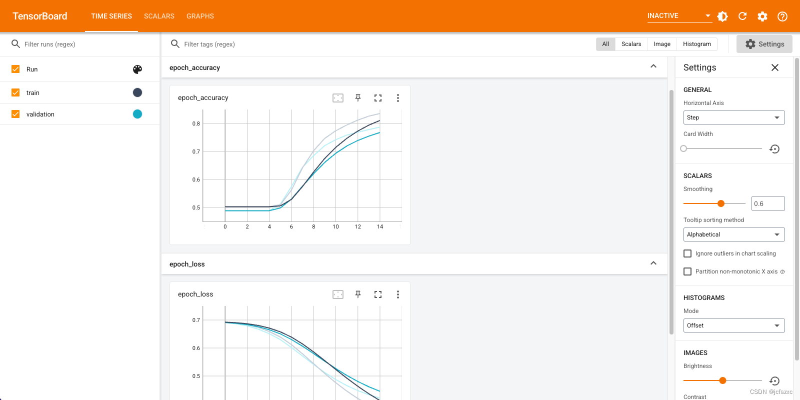
在 TensorBoard 中可视化模型指标。

#docs_infra: no_execute
%load_ext tensorboard
%tensorboard --logdir logs

检索经过训练的单词嵌入并将其保存到磁盘

接下来，检索在训练期间学习的单词嵌入。嵌入是模型中嵌入层的权重。权重矩阵的形状(vocab_size, embedding_dimension)为 。

使用 get_layer() 和 get_weights()从模型中获取权重。该get_vocabulary()函数提供词汇表，用于生成元数据文件，每行一个标记。

weights = model.get_layer('embedding').get_weights()[0]
vocab = vectorize_layer.get_vocabulary()

将权重写入磁盘。要使用嵌入式投影仪，您需要上传两个以制表符分隔的文件：一个向量文件（包含嵌入）和一个元数据文件（包含单词）。

out_v = io.open('vectors.tsv', 'w', encoding='utf-8')
out_m = io.open('metadata.tsv', 'w', encoding='utf-8')

for index, word in enumerate(vocab):
  if index == 0:
    continue  # skip 0, it's padding.
  vec = weights[index]
  out_v.write('\t'.join([str(x) for x in vec]) + "\n")
  out_m.write(word + "\n")
out_v.close()
out_m.close()

如果在 Colaboratory 中运行本教程，可以使用以下代码段将这些文件下载到本地计算机（或使用文件浏览器，查看 -> 目录 -> 文件浏览器）。

try:
  from google.colab import files
  files.download('vectors.tsv')
  files.download('metadata.tsv')
except Exception:
  pass

可视化嵌入

要使嵌入结果可视化，可将其上传到嵌入投影仪。

打开 Embedding Projector（也可在本地 TensorBoard 实例中运行）。

• 点击 “加载数据”。
• 上传上面创建的两个文件：vecs.tsv和meta.tsv。

现在将显示您训练过的嵌入。您可以搜索单词，找到它们的近邻。例如，尝试搜索 “beautiful”。您可能会看到 "美妙 "这样的邻近词。

注：实验证明，使用更简单的模型可能会生成更多可解释的嵌入结果。请尝试删除 Dense(16) 层，重新训练模型，并再次可视化嵌入结果。

注：通常情况下，需要更大的数据集才能训练出更多可解释的词嵌入。本教程使用一个小型 IMDb 数据集进行演示。

下一步工作

本教程向你展示了如何在一个小型数据集上从头开始训练和可视化单词嵌入。

• 要使用 Word2Vec 算法训练单词嵌入，请尝试 Word2Vec 教程。

• 要了解有关高级文本处理的更多信息，请阅读语言理解的 Transformer 模型。