[Optimization] Modeling

Continuos $ Discrete

By default, when we talk about an optimization problem, we assume it is continuous, unless we explicitly say that it is discrete.

1. Continuous Optimization:

   • Nature of Variables: In continuous optimization, the decision variables can take any real value within a specified range. These variables are not restricted to specific values and can vary smoothly.
   • Examples: Problems involving physical quantities like distance, time, temperature, where solutions can be any real number within a given range.
   • Techniques: Gradient-based methods, calculus-based approaches like gradient descent, and mathematical tools like calculus are often used to find optimal solutions.

2. Discrete Optimization:

   • Nature of Variables: Discrete optimization deals with decision variables that can only take distinct, separate values. These values are often integers or belong to a finite set of options.
   • Examples: Combinatorial problems like the traveling salesman problem, where the solution involves selecting a sequence of cities to minimize the total distance traveled.
   • Techniques: Methods like dynamic programming, branch and bound, and integer programming are commonly employed for solving discrete optimization problems.

Linear or Nonlinear

1. Linear Optimization:

   • Objective Function and Constraints: In linear optimization, both the objective function and the constraints are linear functions of the decision variables.
   • Linearity: The term "linear" refers to the fact that each variable is raised to the power of 1 and is multiplied by a constant. The overall relationship between variables is linear.
   • Examples: Linear programming problems, such as maximizing or minimizing a linear objective function subject to linear constraints.

2. Nonlinear Optimization:

   • Objective Function and/or Constraints: In nonlinear optimization, at least one of the objective function or constraints involves nonlinear relationships with the decision variables.
   • Nonlinearity: Nonlinear functions can involve variables raised to powers other than 1, multiplicative combinations of variables, trigonometric functions, exponentials, or other nonlinear mathematical operations.
   • Examples: Optimization problems where the objective function or constraints include terms like x^2, sin(x), e^x, etc.

Modeling is extremely important:

I? ?Finding a good optimization model is at least half way in solving the problem

I? ?In practice, we are not given a mathematical formulation — typically the problem is described verbally by a specialist within some domain. It is extremely important to be able to convert the problem into a mathematical formulation

I? ?Modeling is not trivial: Sometimes, we not only want to find a formulation, but also want to find a good formulation.

The golden rule: Find and formulate the three components

I Decision → Decision variables

I Objective → Objective functions

I Constraints → Constraint functions/inequalities

Ask yourself:

What category this optimization problem belongs to?

Basic acquantance with what would be told

Maximum Area Problem Revisited

You have 80 meters of fencing and want to enclose a rectangle yard as large (area) as possible. How should you do it?

I Decision variable: the length l?and width w of the yard

I Objective: maximize the area: lw

I Constraints: the total length of yard available: 2l + 2w ≤ 80, l,w ≥ 0

Production Problem

Shortest Path Problem

Some notations: We define the set of edges by E. The distance between node i and node j is wij .

Denotations

In this course, we use bold font to denote vectors:?x = (x1, ..., xn).

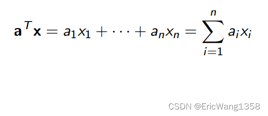
By default, all vectors are column vectors. We use x^T to denote the transpose of a vector.

We use a^T x to denote the inner product of a and x

ex:

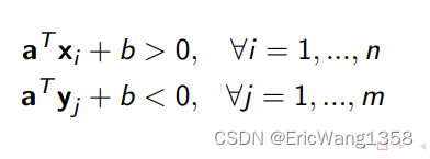
Given two groups of data points in R d , A = {x1, ..., xn} and B = {y1 , ..., ym}. We want to find a plane that separates them.

It is used in pattern recognition, machine learning, etc. Decision: A plane a T x + b = 0 defined by (a, b) that separates the points such that

We call such problems feasibility problems: feasibility problem is a special kind of optimization problem

Sometimes a total separation is not possible:?Then we want to find a plane such that the total “error” is minimized: (we write (w) + for max{w, 0})?（取正部分）

The expression?describe a linear decision boundary in a two-class classification scenario, where we have two sets of points, A and B.?The decision boundary is defined by a hyperplane , where a is the normal vector to the hyperplane, and b is a constant term.The two sets of points are separated by this hyperplane in such a way that points in set A are on one side of the hyperplane? and points in set B are on the other side .

The expressions for all x in set X and? for all y in set Y are considered equivalent conditions.?

（

在这个表达式中， 描述了一个决策边界（decision boundary）在机器学习或优化问题中的应用。让我们解释一下这个表达式中各个部分的含义：

• a 是一个向量，被称为决策边界的法向量（normal vector）。它决定了决策边界的方向。
• xi? 是输入数据的第 i 个样本的特征向量。
• b 是一个常数项，也被称为偏置（bias）或截距（intercept）。

这个表达式实际上表示了样本 xi? 在决策边界上的投影。具体来说：

• 如果 ，则样本 xi? 被分为决策边界的一侧。
• 如果 ，则样本 xi? 被分为决策边界的另一侧。

在一些分类问题中，这个表达式用于判断样本在特征空间中的位置，从而将样本分配到不同的类别。在支持向量机（Support Vector Machine，SVM）等算法中，通过调整 a 和 b 的取值，可以找到一个最优的决策边界，以便在两个类别之间进行有效的分类。

在一些优化问题和分类算法中，对于决策边界的具体形式，可以使用 或 ，通常具体的选择取决于问题的要求和算法的设计。

在支持向量机（Support Vector Machine，SVM）等算法中，常常使用?，这是因为这样的选择使得决策边界更加“宽阔”（wide margin），有助于提高模型的泛化性能。通过调整 a 和 b 的取值，可以找到一个最大间隔的决策边界，以更好地区分不同类别的样本。在实际应用中，有时为了简化问题，也可以使用??特别是当问题的复杂性不要求很大的间隔时。这在一些问题中可能会导致相似的效果，但在对于决策边界的选择上，具体的取值通常需要根据具体的问题和算法的设计来确定。

）

For points in A, the error is?，

For points in B, the error is?，

（即如果大于零，那么误差为零，否则误差为或）

Therefore we can write the support vector machine problem as:

This is an unconstrained, nonlinear, continuous optimization problem.

Define?，

The relaxed problem is more amenable to optimization techniques.?The solutions to the relaxed problem will satisfy the original equalities。（You have an optimization problem where you want to find the values of a and b that minimize a certain expression involving δi? and σj?. These δi? and σj? are related to the differences between the actual values and the predicted values in your model. Originally, you said these differences must be exactly zero (equality). However, sometimes it's easier to solve problems when you allow a little flexibility. So, instead of insisting that these differences are exactly zero, you relax the requirement and say they just need to be greater than or equal to zero.）

why it (relaxing) makes it easier to solve problems?

1. Convexity:

   • In many cases, the relaxed problem becomes convex. Convex optimization problems have well-established algorithms and properties that make them computationally more tractable.
   • The positive part operation (?)+(?)+ introduces piecewise linearity, which preserves convexity.

2. Broader Solution Space:

   • Equality constraints can make the solution space more restrictive, limiting the possibilities for finding an optimal solution.
   • Inequalities allow for a broader range of solutions, making it more likely to find a global optimum.

3. Numerical Stability:

   • Numerical algorithms for solving optimization problems often perform more stably with inequalities. Equality constraints can sometimes lead to numerical issues.

4. Feasibility:

   • Relaxing to inequalities ensures that the solution space is feasible, meaning there is a greater likelihood of finding a solution that satisfies the optimization problem.

5. Computational Efficiency:

   • Algorithms for solving convex optimization problems are well-developed and efficient. By formulating the problem with convex inequalities, you can leverage these algorithms.

6. Simplification of Expressions:

   • Inequality constraints can lead to simpler expressions and mathematical formulations, making it easier to work with and understand the optimization problem.

And finally,?the optimization problem can be transformed to

为什么变量是这四个 然后就linear了？

the equations about?, a,b , ?are linear inequalities.