【Pytorch】学习记录分享4——PyTorch 天气预测线性回归实例

1. hub使用教程

视频B站链接教程
官网教程：

2. 结构性数据加载

2.1 数据格式入下

数据表中
year,moth,day,week分别表示的具体的时间
temp_2：前天的最高温度值
temp_1：昨天的最高温度值
average：在历史中，每年这一天的平均最高温度值
actual：这就是我们的标签值了，当天的真实最高温度
friend：这一列可能是凑热闹的，你的朋友猜测的可能值

year,month,day,week,temp_2,temp_1,average,actual,friend
2016,1,1,Fri,45,45,45.6,45,29
2016,1,2,Sat,44,45,45.7,44,61
2016,1,3,Sun,45,44,45.8,41,56
2016,1,4,Mon,44,41,45.9,40,53
2016,1,5,Tues,41,40,46,44,41
2016,1,6,Wed,40,44,46.1,51,40
......

import numpy as np
import pandas as pd 
import matplotlib.pyplot as plt
import torch
import torch.optim as optim
import warnings
warnings.filterwarnings("ignore")
%matplotlib inline

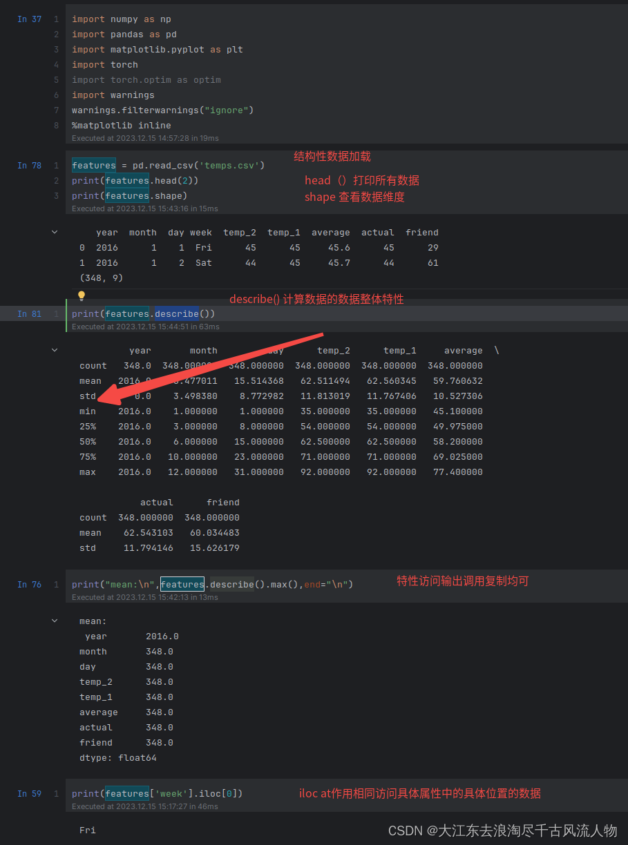
features = pd.read_csv('temps.csv')
print(features.head(2))
print(features.shape)

print(features.describe())
print("mean:\n",features.describe().max(),end="\n")
print(features['week'].iloc[0])
print(features.groupby(['week']).mean())
#看看数据长什么样子
features.head()
print('数据维度:', features.shape)

3 结构性数据显示

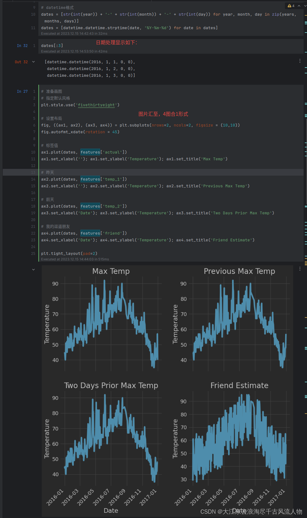
# 处理时间数据
import datetime

# 分别得到年，月，日
years = features['year']
months = features['month']
days = features['day']

# datetime格式
dates = [str(int(year)) + '-' + str(int(month)) + '-' + str(int(day)) for year, month, day in zip(years, months, days)]
dates = [datetime.datetime.strptime(date, '%Y-%m-%d') for date in dates]

dates[:3]

# 准备画图
# 指定默认风格
plt.style.use('fivethirtyeight')

# 设置布局
fig, ((ax1, ax2), (ax3, ax4)) = plt.subplots(nrows=2, ncols=2, figsize = (10,10))
fig.autofmt_xdate(rotation = 45)

# 标签值
ax1.plot(dates, features['actual'])
ax1.set_xlabel(''); ax1.set_ylabel('Temperature'); ax1.set_title('Max Temp')

# 昨天
ax2.plot(dates, features['temp_1'])
ax2.set_xlabel(''); ax2.set_ylabel('Temperature'); ax2.set_title('Previous Max Temp')

# 前天
ax3.plot(dates, features['temp_2'])
ax3.set_xlabel('Date'); ax3.set_ylabel('Temperature'); ax3.set_title('Two Days Prior Max Temp')

# 我的逗逼朋友
ax4.plot(dates, features['friend'])
ax4.set_xlabel('Date'); ax4.set_ylabel('Temperature'); ax4.set_title('Friend Estimate')

plt.tight_layout(pad=2)

4 结构性数据预处理

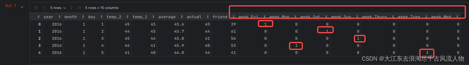
# 独热编码
features = pd.get_dummies(features)
features.head(5)

独热编码是一种用于处理分类变量的方法，它将一个具有n个可能取值的分类变量转换成n个新的二元变量，每个二元变量代表了原始变量中的一个可能取值。这样做的好处是在使用机器学习算法时，可以更好地处理分类变量，因为大部分机器学习算法更适合处理数值型数据。

实现方法：

1. 找到数据中的所有分类变量。
2. 对每个分类变量的每个可能取值，创建一个新的二元变量，表示原始变量中的某个取值是否存在。
3. 删除原始的分类变量列，保留新生成的二元变量列。

例如，对于一个“性别”这样的分类变量，如果原始数据中有"男"和"女"两种取值，经过独热编码处理后，会生成两个新的二元变量列"性别_男"和"性别_女"，其中每行的值为1或0来表示原始数据中的性别情况。如果是星期几的话，编码后如下图所示：

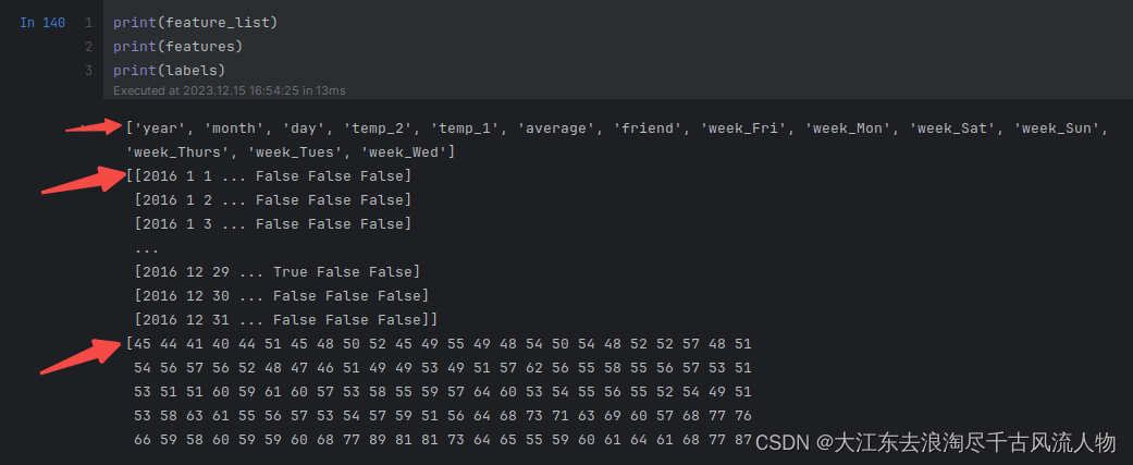
去除features数据中的真值，保存到labels中，并且在特征中去掉标签列

# 标签
labels = np.array(features['actual'])

# 在特征中去掉标签
features= features.drop('actual', axis = 1)

# 名字单独保存一下，以备后患
feature_list = list(features.columns)

# 转换成合适的格式
features = np.array(features)

features.shape

print(feature_list)
print(features)
print(labels)

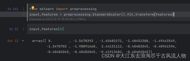
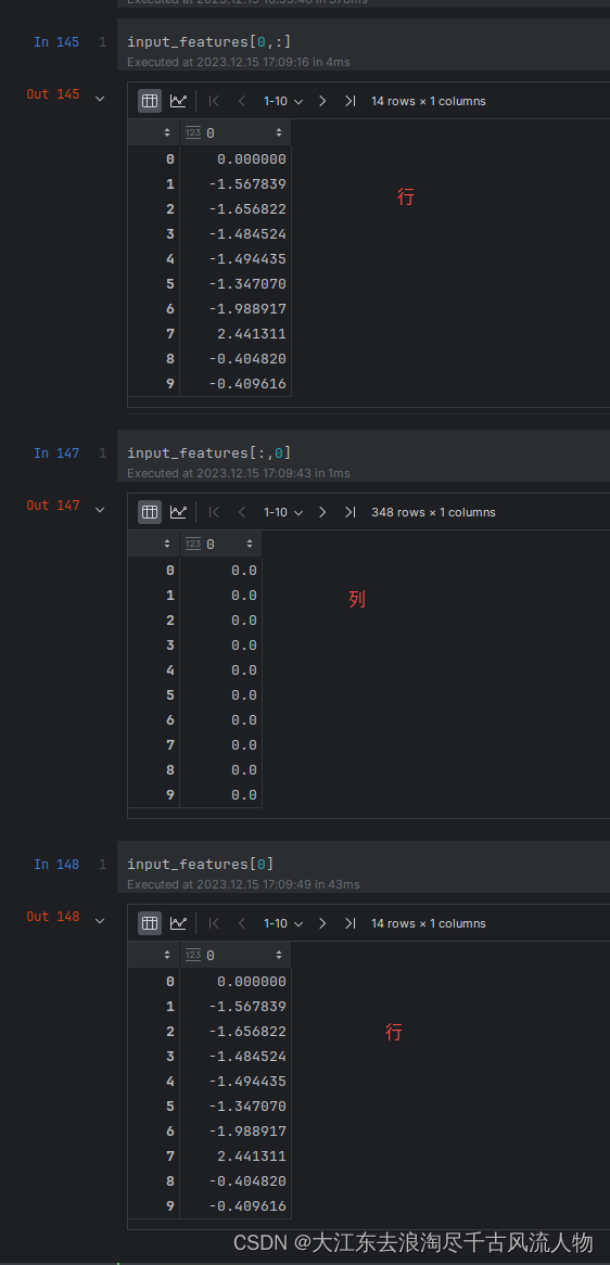
from sklearn import preprocessing
input_features = preprocessing.StandardScaler().fit_transform(features)

这行代码使用StandardScaler对特征进行标准化处理，包括均值移除和方差缩放，使得特征的均值为0，方差为1。fit_transform
方法用于对数据集进行拟合转换操作，将处理后的结果存储在input_features中。

4 网络模型构建

4.1 方法1

x = torch.tensor(input_features, dtype = float)

y = torch.tensor(labels, dtype = float)

# 权重参数初始化
weights = torch.randn((14, 128), dtype = float, requires_grad = True) 
biases = torch.randn(128, dtype = float, requires_grad = True) 
weights2 = torch.randn((128, 1), dtype = float, requires_grad = True) 
biases2 = torch.randn(1, dtype = float, requires_grad = True) 

learning_rate = 0.001 
losses = []

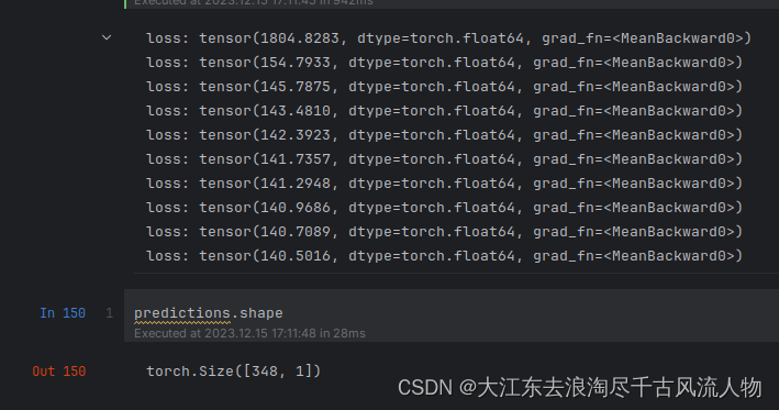
for i in range(1000):
    # 计算隐层
    hidden = x.mm(weights) + biases
    # 加入激活函数
    hidden = torch.relu(hidden)
    # 预测结果
    predictions = hidden.mm(weights2) + biases2
    # 通计算损失
    loss = torch.mean((predictions - y) ** 2) 
    losses.append(loss.data.numpy())
    
    # 打印损失值
    if i % 100 == 0:
        print('loss:', loss)
    #返向传播计算
    loss.backward()
    
    #更新参数
    weights.data.add_(- learning_rate * weights.grad.data)  
    biases.data.add_(- learning_rate * biases.grad.data)
    weights2.data.add_(- learning_rate * weights2.grad.data)
    biases2.data.add_(- learning_rate * biases2.grad.data)
    
    # 每次迭代都得记得清空
    weights.grad.data.zero_()
    biases.grad.data.zero_()
    weights2.grad.data.zero_()
    biases2.grad.data.zero_()

predictions.shape

4.1 方法2（更简单的构建网络模型）

input_size = input_features.shape[1]
hidden_size = 128
output_size = 1
batch_size = 16
my_nn = torch.nn.Sequential(
    torch.nn.Linear(input_size, hidden_size),
    torch.nn.Sigmoid(),
    torch.nn.Linear(hidden_size, output_size),
)
cost = torch.nn.MSELoss(reduction='mean')
optimizer = torch.optim.Adam(my_nn.parameters(), lr = 0.001)

# 训练网络
losses = []
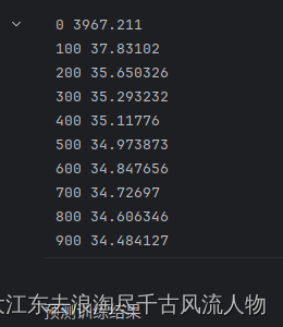
for i in range(1000):
    batch_loss = []
    # MINI-Batch方法来进行训练
    for start in range(0, len(input_features), batch_size):
        end = start + batch_size if start + batch_size < len(input_features) else len(input_features)
        xx = torch.tensor(input_features[start:end], dtype = torch.float, requires_grad = True)
        yy = torch.tensor(labels[start:end], dtype = torch.float, requires_grad = True)
        prediction = my_nn(xx)
        loss = cost(prediction, yy)
        optimizer.zero_grad()
        loss.backward(retain_graph=True)
        optimizer.step()
        batch_loss.append(loss.data.numpy())
    
    # 打印损失
    if i % 100==0:
        losses.append(np.mean(batch_loss))
        print(i, np.mean(batch_loss))

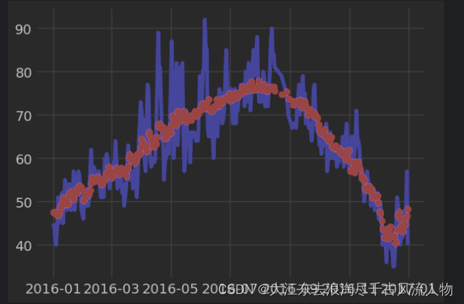
5. 网络模型预测使用测试

x = torch.tensor(input_features, dtype = torch.float)
predict = my_nn(x).data.numpy()

# 转换日期格式
dates = [str(int(year)) + '-' + str(int(month)) + '-' + str(int(day)) for year, month, day in zip(years, months, days)]
dates = [datetime.datetime.strptime(date, '%Y-%m-%d') for date in dates]

# 创建一个表格来存日期和其对应的标签数值
true_data = pd.DataFrame(data = {'date': dates, 'actual': labels})

# 同理，再创建一个来存日期和其对应的模型预测值
months = features[:, feature_list.index('month')]
days = features[:, feature_list.index('day')]
years = features[:, feature_list.index('year')]

test_dates = [str(int(year)) + '-' + str(int(month)) + '-' + str(int(day)) for year, month, day in zip(years, months, days)]

test_dates = [datetime.datetime.strptime(date, '%Y-%m-%d') for date in test_dates]

predictions_data = pd.DataFrame(data = {'date': test_dates, 'prediction': predict.reshape(-1)}) 

# 真实值
plt.plot(true_data['date'], true_data['actual'], 'b-', label = 'actual')

# 预测值
plt.plot(predictions_data['date'], predictions_data['prediction'], 'ro', label = 'prediction')
plt.xticks(rotation = '60'); 
plt.legend()

# 图名
plt.xlabel('Date'); plt.ylabel('Maximum Temperature (F)'); plt.title('Actual and Predicted Values');