助力打造智慧数字课堂，基于YOLOv6开发构建教学课堂场景下学生课堂行为检测识别分析系统

近年来，随着行为检测技术的发展，分析学生在课堂视频中的行为，以获取他们的课堂状态和学习表现信息已经成为可能。这项技术对学校的教师、管理人员、学生和家长都非常重要。使用深度学习方法自动检测学生的课堂行为是分析学生课堂表现和提高教学效果的一种很有前途的方法。在传统的教学模式中，教师很难及时有效地关注每个学生的学习情况，只能通过观察少数学生来了解自己教学方法的有效性。加之课堂时间有效提问式的交互方式难以覆盖到所有人群，传统的应试教育模式通过考试来检查学生知识掌握的程度往往具有滞后性和低效性。除此之外，学生家长只有通过与老师和学生的交流才能了解孩子的学习情况。而这些反馈相对具有主观性，学习本身是一个需要自发性主动性去参与的过程，但是在青春的年纪很多学习之外的诱惑或者是注意力不集中等因素会导致学生在课堂的参与度不高，如何通过教学过程中的及时反馈响应来聚焦课堂注意力提高教学效率成为了最核心的问题，我们不是教育专家，我们只是喜欢探讨如何将技术与现实生活场景相结合，本文的核心思想就是想要探索利用目标检测模型来检测分析学生的行为，分析他们的学习状态和表现，对于出现的异常行为进行响应或者是记录，为教育教学提供更全面、准确的反馈，通过对课堂行为数据的分析进而有效地纠正低效的课堂行为，从而提高学习成绩。

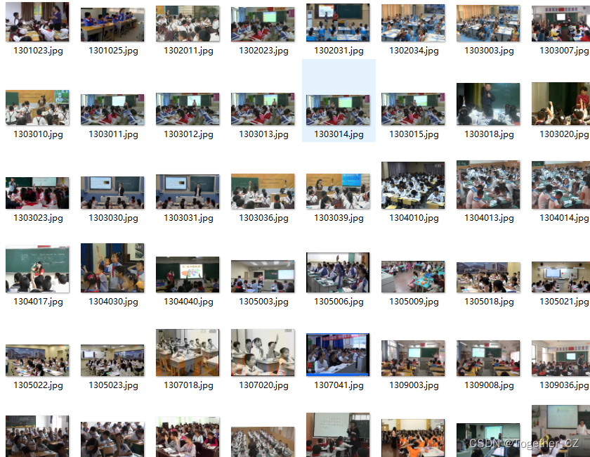
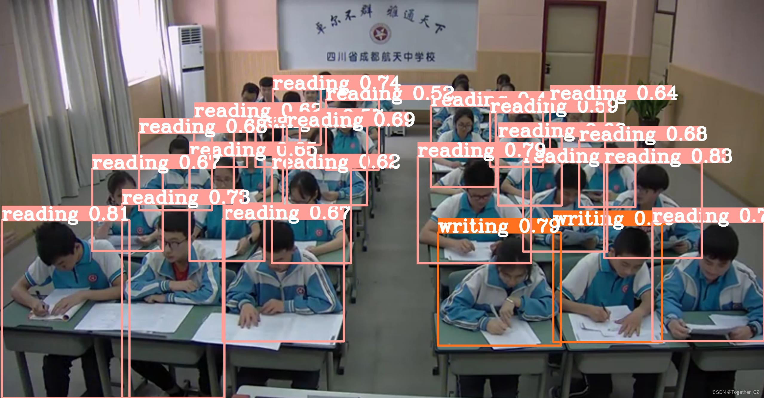
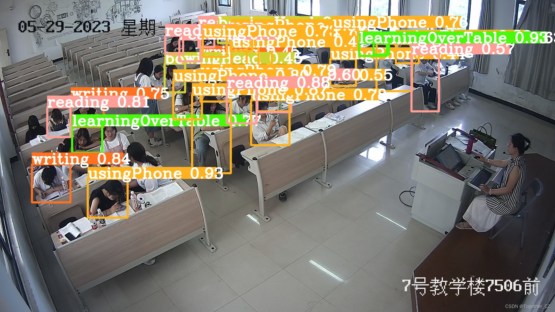
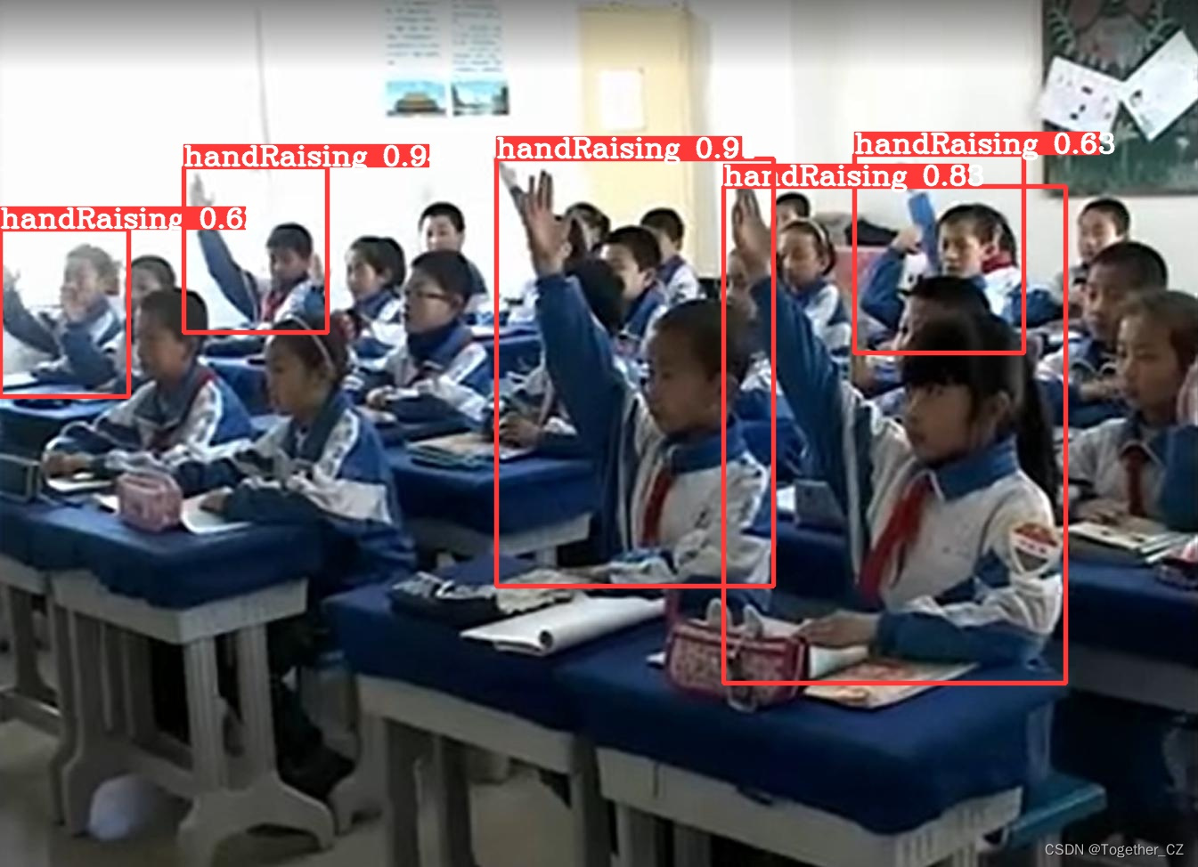
本文主要是选择最新的YOLOv6来开发实现检测模型，我们开发了n和s两款不同参数量级的模型用于整体对比分析，首先看下实例效果：

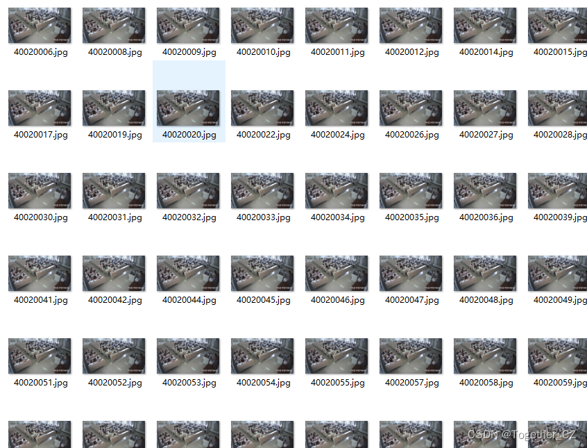
简单看下实例数据情况：

在前文中我们已经进行了相关的项目开发实践，感兴趣的话可以自行移步阅读：

《助力打造智慧数字课堂，基于YOLOv5全系列【n/s/m/l/x】不同参数量级模型开发构建教学课堂场景下学生课堂行为检测识别分析系统》

《助力打造智慧数字课堂，基于YOLOv8全系列【n/s/m/l/x】不同参数量级模型开发构建教学课堂场景下学生课堂行为检测识别分析系统》

Yolov6是美团开发的轻量级检测算法，截至目前为止该算法已经迭代到了4.0版本，每一个版本都包含了当时最优秀的检测技巧和最最先进的技术，YOLOv6的Backbone不再使用Cspdarknet，而是转为比Rep更高效的EfficientRep；它的Neck也是基于Rep和PAN搭建了Rep-PAN；而Head则和YOLOX一样，进行了解耦，并且加入了更为高效的结构。YOLOv6也是沿用anchor-free的方式，抛弃了以前基于anchor的方法。除了模型的结构之外，它的数据增强和YOLOv5的保持一致；而标签分配上则是和YOLOX一样，采用了simOTA；并且引入了新的边框回归损失：SIOU。
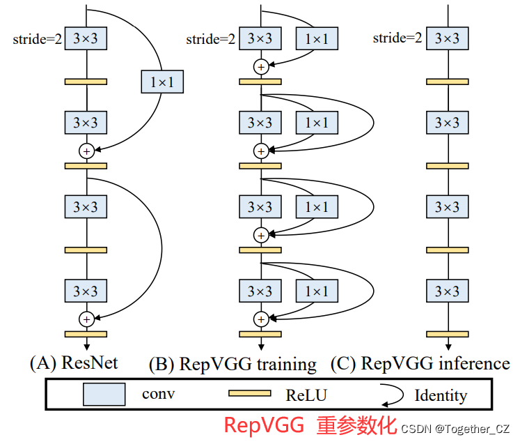
YOLOv5和YOLOX都是采用多分支的残差结构CSPNet，但是这种结构对于硬件来说并不是很友好。所以为了更加适应GPU设备，在backbone上就引入了ReVGG的结构，并且基于硬件又进行了改良，提出了效率更高的EfficientRep。RepVGG为每一个3×3的卷积添加平行了一个1x1的卷积分支和恒等映射的分支。这种结构就构成了构成一个RepVGG Block。和ResNet不同的是，RepVGG是每一层都添加这种结构，而ResNet是每隔两层或者三层才添加。RepVGG介绍称，通过融合而成的3x3卷积结构，对计算密集型的硬件设备很友好。
?

如果大家对于如何使用美团开源的YOLOv6来开发构建自己的个性化目标检测应用，可以评论区留言，我来做一期超详细的实战教程。

训练数据配置文件如下所示：

# Please insure that your custom_dataset are put in same parent dir with YOLOv6_DIR
train: ./dataset/images/train # train images
val: ./dataset/images/test # val images
test: ./dataset/images/test # test images (optional)

# whether it is coco dataset, only coco dataset should be set to True.
is_coco: False

# Classes
nc: 6  # number of classes

# class names
names: ['handRaising', 'reading', 'writing', 'usingPhone', 'bowingHead', 'learningOverTable']

这里我们一共开发了两款不同量级的模型，分别是yolov6n和yolov6s，两款模型都是基于finetune来进行模型的开发：

【yolov6n】

# YOLOv6s model
model = dict(
    type='YOLOv6n',
    pretrained='weights/yolov6n.pt',
    depth_multiple=0.33,
    width_multiple=0.25,
    backbone=dict(
        type='EfficientRep',
        num_repeats=[1, 6, 12, 18, 6],
        out_channels=[64, 128, 256, 512, 1024],
        fuse_P2=True,
        cspsppf=True,
        ),
    neck=dict(
        type='RepBiFPANNeck',
        num_repeats=[12, 12, 12, 12],
        out_channels=[256, 128, 128, 256, 256, 512],
        ),
    head=dict(
        type='EffiDeHead',
        in_channels=[128, 256, 512],
        num_layers=3,
        begin_indices=24,
        anchors=3,
        anchors_init=[[10,13, 19,19, 33,23],
                      [30,61, 59,59, 59,119],
                      [116,90, 185,185, 373,326]],
        out_indices=[17, 20, 23],
        strides=[8, 16, 32],
        atss_warmup_epoch=0,
        iou_type='siou',
        use_dfl=False, # set to True if you want to further train with distillation
        reg_max=0, # set to 16 if you want to further train with distillation
        distill_weight={
            'class': 1.0,
            'dfl': 1.0,
        },
    )
)

solver = dict(
    optim='SGD',
    lr_scheduler='Cosine',
    lr0=0.0032,
    lrf=0.12,
    momentum=0.843,
    weight_decay=0.00036,
    warmup_epochs=2.0,
    warmup_momentum=0.5,
    warmup_bias_lr=0.05
)

data_aug = dict(
    hsv_h=0.0138,
    hsv_s=0.664,
    hsv_v=0.464,
    degrees=0.373,
    translate=0.245,
    scale=0.898,
    shear=0.602,
    flipud=0.00856,
    fliplr=0.5,
    mosaic=1.0,
    mixup=0.243,
)

【yolov6s】

# YOLOv6s model
model = dict(
    type='YOLOv6s',
    pretrained='weights/yolov6s.pt',
    depth_multiple=0.33,
    width_multiple=0.50,
    backbone=dict(
        type='EfficientRep',
        num_repeats=[1, 6, 12, 18, 6],
        out_channels=[64, 128, 256, 512, 1024],
        fuse_P2=True,
        cspsppf=True,
        ),
    neck=dict(
        type='RepBiFPANNeck',
        num_repeats=[12, 12, 12, 12],
        out_channels=[256, 128, 128, 256, 256, 512],
        ),
    head=dict(
        type='EffiDeHead',
        in_channels=[128, 256, 512],
        num_layers=3,
        begin_indices=24,
        anchors=3,
        anchors_init=[[10,13, 19,19, 33,23],
                      [30,61, 59,59, 59,119],
                      [116,90, 185,185, 373,326]],
        out_indices=[17, 20, 23],
        strides=[8, 16, 32],
        atss_warmup_epoch=0,
        iou_type='giou',
        use_dfl=False, # set to True if you want to further train with distillation
        reg_max=0, # set to 16 if you want to further train with distillation
        distill_weight={
            'class': 1.0,
            'dfl': 1.0,
        },
    )
)

solver = dict(
    optim='SGD',
    lr_scheduler='Cosine',
    lr0=0.0032,
    lrf=0.12,
    momentum=0.843,
    weight_decay=0.00036,
    warmup_epochs=2.0,
    warmup_momentum=0.5,
    warmup_bias_lr=0.05
)

data_aug = dict(
    hsv_h=0.0138,
    hsv_s=0.664,
    hsv_v=0.464,
    degrees=0.373,
    translate=0.245,
    scale=0.898,
    shear=0.602,
    flipud=0.00856,
    fliplr=0.5,
    mosaic=1.0,
    mixup=0.243,
)

终端执行：

【yolov6n】
python3 tools/train.py --batch-size 16 --conf configs/yolov6n_finetune.py --data data/self.yaml --fuse_ab --device 0 --name yolov6n --epochs 100 --workers 2


【yolov6s】
python3 tools/train.py --batch-size 16 --conf configs/yolov6s_finetune.py --data data/self.yaml --fuse_ab --device 0 --name yolov6s --epochs 100 --workers 2

终端日志输出如下所示：

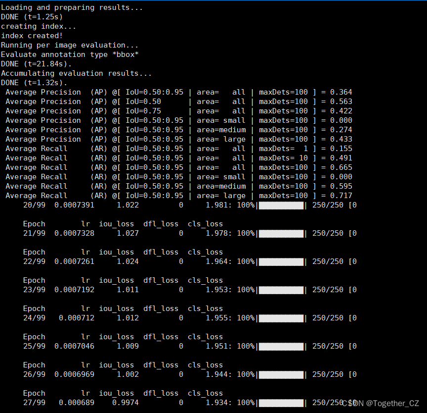
训练完成输出如下所示：

【yolov6n】
Training completed in 3.786 hours.
loading annotations into memory...
Done (t=0.04s)
creating index...
index created!
Loading and preparing results...
DONE (t=1.16s)
creating index...
index created!
Running per image evaluation...
Evaluate annotation type *bbox*
DONE (t=20.95s).
Accumulating evaluation results...
DONE (t=1.24s).
 Average Precision  (AP) @[ IoU=0.50:0.95 | area=   all | maxDets=100 ] = 0.530
 Average Precision  (AP) @[ IoU=0.50      | area=   all | maxDets=100 ] = 0.767
 Average Precision  (AP) @[ IoU=0.75      | area=   all | maxDets=100 ] = 0.614
 Average Precision  (AP) @[ IoU=0.50:0.95 | area= small | maxDets=100 ] = 0.000
 Average Precision  (AP) @[ IoU=0.50:0.95 | area=medium | maxDets=100 ] = 0.434
 Average Precision  (AP) @[ IoU=0.50:0.95 | area= large | maxDets=100 ] = 0.598
 Average Recall     (AR) @[ IoU=0.50:0.95 | area=   all | maxDets=  1 ] = 0.205
 Average Recall     (AR) @[ IoU=0.50:0.95 | area=   all | maxDets= 10 ] = 0.592
 Average Recall     (AR) @[ IoU=0.50:0.95 | area=   all | maxDets=100 ] = 0.724
 Average Recall     (AR) @[ IoU=0.50:0.95 | area= small | maxDets=100 ] = 0.000
 Average Recall     (AR) @[ IoU=0.50:0.95 | area=medium | maxDets=100 ] = 0.656
 Average Recall     (AR) @[ IoU=0.50:0.95 | area= large | maxDets=100 ] = 0.782


【yolov6s】
Training completed in 10.869 hours.
loading annotations into memory...
Done (t=0.18s)
creating index...
index created!
Loading and preparing results...
DONE (t=0.82s)
creating index...
index created!
Running per image evaluation...
Evaluate annotation type *bbox*
DONE (t=19.91s).
Accumulating evaluation results...
DONE (t=1.10s).
 Average Precision  (AP) @[ IoU=0.50:0.95 | area=   all | maxDets=100 ] = 0.658
 Average Precision  (AP) @[ IoU=0.50      | area=   all | maxDets=100 ] = 0.871
 Average Precision  (AP) @[ IoU=0.75      | area=   all | maxDets=100 ] = 0.786
 Average Precision  (AP) @[ IoU=0.50:0.95 | area= small | maxDets=100 ] = 0.000
 Average Precision  (AP) @[ IoU=0.50:0.95 | area=medium | maxDets=100 ] = 0.594
 Average Precision  (AP) @[ IoU=0.50:0.95 | area= large | maxDets=100 ] = 0.709
 Average Recall     (AR) @[ IoU=0.50:0.95 | area=   all | maxDets=  1 ] = 0.232
 Average Recall     (AR) @[ IoU=0.50:0.95 | area=   all | maxDets= 10 ] = 0.686
 Average Recall     (AR) @[ IoU=0.50:0.95 | area=   all | maxDets=100 ] = 0.793
 Average Recall     (AR) @[ IoU=0.50:0.95 | area= small | maxDets=100 ] = 0.000
 Average Recall     (AR) @[ IoU=0.50:0.95 | area=medium | maxDets=100 ] = 0.739
 Average Recall     (AR) @[ IoU=0.50:0.95 | area= large | maxDets=100 ] = 0.839

从指标对比来看：s模型的效果要优于n系列不少。

这里我们就选定使用s模型作为基准推理模型，离线推理实例如下所示：

效果还不错，后期我们要对几款不同的模型来综合对比选择，等到后面全部完成后抽时间再来评测吧。