[Probability] 1.5 story proof and non-naive def

A story proof is a proof by interpretation.

For counting problems, this often means counting the same thing in two different ways, rather than doing tedious algebra. A story proof often avoids messy calculations and goes further than an algebraic proof toward explaining why the result is true.

The word “story” has several meanings, some more mathematical than others, but a story proof (in the sense in which we’re using the term) is a fully valid mathematical proof. Here are some examples of story proofs, which also serve as further examples of counting.

(Choosing the complement) n choose k = n choose n-k

(The team captain)?

For any positive integers n and k with k ≤ n, n( n-1 choose k-1) = k (n choose k)

This is again easy to check algebraically (using the fact that m! = m(m ? 1)! for any positive integer m), but a story proof is more insightful.

Story proof : Consider a group of n people, from which a team of k will be chosen, one of whom will be the team captain. To specify a possibility, we could first choose the team captain and then choose the remaining k ? 1 team members; this gives the left-hand side. Equivalently, we could first choose the k team members and then choose one of them to be captain; this gives the right-hand side

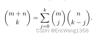
(Vandermonde’s identity)

A famous relationship between binomial coefficients, called Vandermonde’s identity

Consider a student organization consisting of m juniors and n seniors, from which a committee of size k will be chosen. There are (m+n choose k)?possibilities. If there are j juniors in the committee, then there must be k ? j seniors in the committee. The right-hand side of the identity sums up the cases for j.

(Partnerships).

We can form partnerships by lining up the people in some order and then saying the first two are a pair, the next two are a pair, etc.?

Non-naive definition of probability

Definition 1.6.1 (General definition of probability).

A probability space consists of a sample space S and a probability function P which takes an event A ? S as input and returns P(A), a real number between 0 and 1, as output. The function P must satisfy the following axioms:

Unlike in the naive case, we can now have pebbles of differing masses, and we can also have a countably infinite number of pebbles as long as their total mass is 1.

We can even have uncountable sample spaces, such as having S be an area in the plane. In this case, instead of pebbles, we can visualize mud spread out over a region, where the total mass of the mud is 1.

However, the axioms don’t tell us how probability should be interpreted; different schools of thought exist.

The frequentist view of probability is that it represents a long-run frequency over a large number of repetitions of an experiment.

The Bayesian view of probability is that it represents a degree of belief about the event in question, so we can assign probabilities to hypotheses.

The Bayesian and frequentist perspectives are complementary. Can be used in

(Properties of probability)

(Inclusion-exclusion)

(de Montmort’s matching problem)