[Probability] 1. Introduction to probability

Why study probability?

A: Probability is the logic of uncertainty. Probability provides procedures for principled problem-solving, but it can also produce pitfalls and paradoxes.

Sample spaces and Pebble World

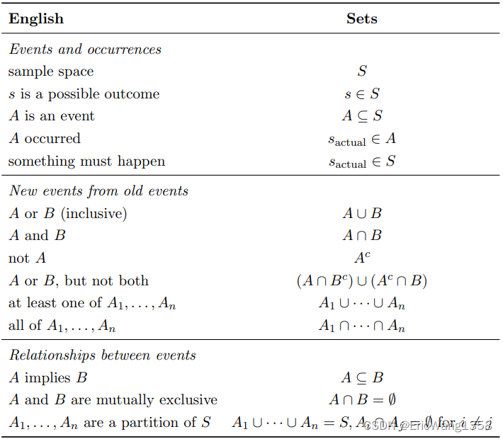
Definition 1.2.1 (Sample space and event). The sample space S of an experiment is the set of all possible outcomes of the experiment. An event A is a subset of the sample space S, and we say that A occurred if the actual outcome is in A

The sample space of an experiment can be finite, countably infinite, or uncountably infinite (an explanation of countable and uncountable sets). When the sample space is finite, we can visualize it as Pebble World. Each pebble represents an outcome, and an event is a set of pebbles.

What is a countable set?

Question 1:
What is a countable set?

Answer 1:
A countable set is a set that has the same cardinality (size) as the set of natural numbers (1, 2, 3, ...). It can either be finite or have an infinite number of elements, but these elements can be put into a one-to-one correspondence with the natural numbers.

What is an uncountable set?

An uncountable set is a set that is not countable, meaning its elements cannot be put into a one-to-one correspondence with the natural numbers. Uncountable sets have cardinalities greater than that of the set of natural numbers.

The set of real numbers between 0 and 1 is an example of an uncountable set. This set includes an infinite number of elements, and it is not possible to list them in a way that corresponds to the natural numbers.

Countable sets have cardinalities that match the size of the set of natural numbers (?0?), while uncountable sets have cardinalities greater than ?0?.

De Morgan’s laws

?1.3 Naive definition of probability

Definition 1.3.1 (Naive definition of probability). Let A be an event for an experiment with a finite sample space S. The naive probability of A is

?

The naive definition is very restrictive in that it requires S to be finite, with equal mass for each pebble.?

It has often been misapplied by people who assume equally likely outcomes without justification and make arguments to the effect of “either it will happen or it won’t, and we don’t know which, so it’s 50-50”

there are several important types of problems where the naive definition is applicable:

when there is symmetry in the problem that makes outcomes equally likely. It is common to assume that a coin has a 50% chance of landing Heads when tossed, due to the physical symmetry of the coin.1

when the outcomes are equally likely by design.

when the naive definition serves as a useful null model. In this setting, we assume that the naive definition applies just to what predictions it would yield, and then we can compare observed data with predicted values to assess whether the hypothesis of equally likely outcomes is tenable.

Example with Easy Language For Naive definition:

Imagine you have a bag of colored marbles, and you want to see if one color is more common than the others. The naive definition here would be to assume that all colors are equally likely, without any special reason to think otherwise.

The naive definition, in this case, serves as a useful null model. It's like saying, "Well, if everything is random and each color is equally likely, what would we expect to happen just by chance?" So, the naive definition acts as a simple baseline or null hypothesis that helps you gauge whether your observations are surprising or if there might be more going on than just randomness.

1.4 How to count

Theorem 1.4.1 (Multiplication rule).

Consider a compound experiment consisting of two sub-experiments, Experiment A and Experiment B. Suppose that Experiment A has a possible outcomes, and for each of those outcomes Experiment B has b possible outcomes. Then the compound experiment has ab possible outcomes.

h 1.4.2. It is often easier to think about the experiments as being in chronological order, but there is no requirement in the multiplication rule that Experiment A has to be performed before Experiment B.

1.4.2 Adjusting for overcounting

In many counting problems, it is not easy to directly count each possibility once and only once. If, however, we are able to count each possibility exactly c times Probability and counting 15 for some c, then we can adjust by dividing by c. For example, if we have exactly double-counted each possibility, we can divide by 2 to get the correct count. We call this adjusting for overcounting

Definition 1.4.14 (Binomial coefficient).

For any nonnegative integers k and n, the binomial coefficient? (n k) read as “n choose k”, is the number of subsets of size k for a set of size n.

if k > n, it is 0.

Bose-Einstein encoding:

putting k = 7 indistinguishable particles into n = 4 distinguishable boxes can be expressed as a sequence of |’s and ●’s, where | denotes a wall and ● denotes a particle

the number of possibilities is?n+k-1 choose k

The Bose-Einstein result should not be used in the naive definition of probability except in very special circumstances. For example, consider a survey where a sample of size k is collected by choosing people from a population of size n?one at a time, with replacement and with equal probabilities. Then the n^k ordered samples are equally likely, making the naive definition applicable, but the?n+k-1 choose k?unordered samples (where all that matters is how many times each person was sampled) are not equally likely.

Equally likely or Having?the same chance of occurring:

For example, if n = 3 (people A, B, C) and k = 2, then the ordered samples (AB, AC, BA, BC, CA, CB) are all equally likely.

While for n choos k, some combinations might be more likely than others due to the repeated sampling with replacement.