机器学习~从入门到精通（二）线性回归算法和多元线性回归

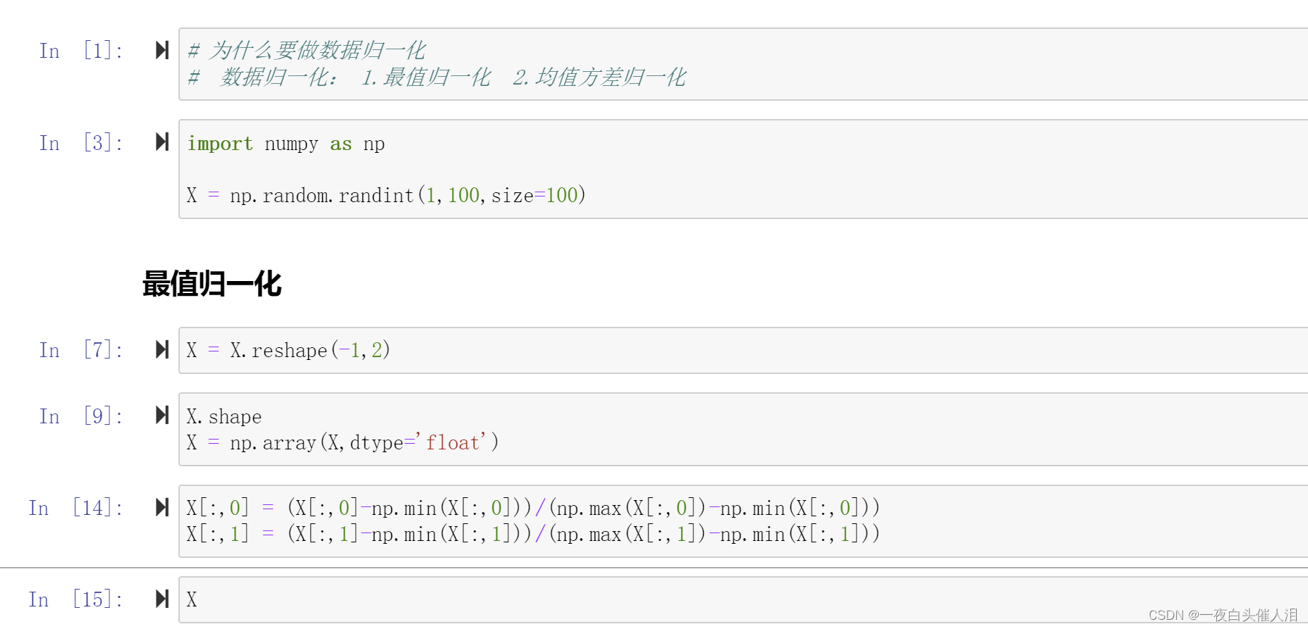
为什么要做数据归一化

一、数据归一化：

1.最值归一化
2.均值方差归一化

import numpy as np

X = np.random.randint(1,100,size=100)
X = X.reshape(-1,2)
X.shape
X = np.array(X,dtype='float')
X[:,0] = (X[:,0]-np.min(X[:,0]))/(np.max(X[:,0])-np.min(X[:,0]))
X[:,1] = (X[:,1]-np.min(X[:,1]))/(np.max(X[:,1])-np.min(X[:,1]))
X

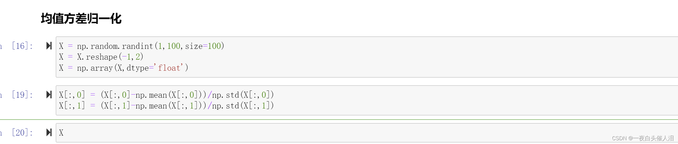
均值方差归一化

X = np.random.randint(1,100,size=100)
X = X.reshape(-1,2)
X = np.array(X,dtype='float')
X[:,0] = (X[:,0]-np.mean(X[:,0]))/np.std(X[:,0])
X[:,1] = (X[:,1]-np.mean(X[:,1]))/np.std(X[:,1])
X

np.std(X[:,0])
np.std(X[:,1])
np.mean(X[:,0])
np.mean(X[:,1])

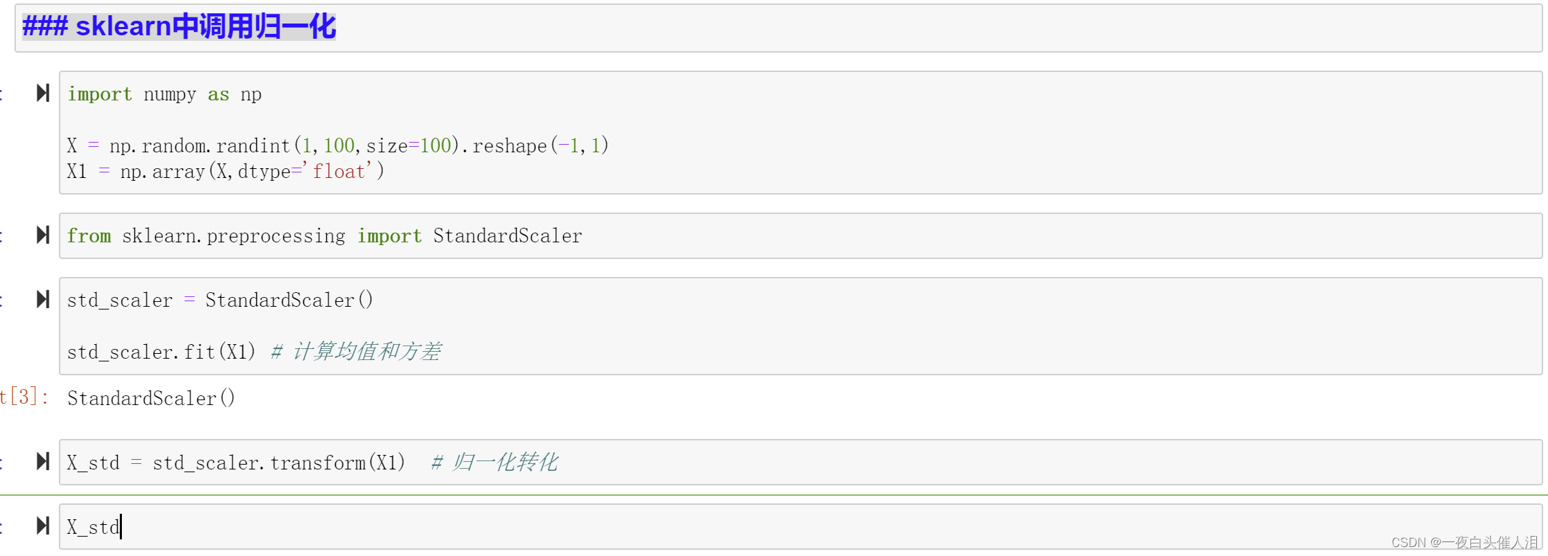
二、数据归一化的注意事项

import numpy as np

X = np.random.randint(1,100,size=100).reshape(-1,1)
X1 = np.array(X,dtype='float')

from sklearn.preprocessing import StandardScaler
std_scaler = StandardScaler()

std_scaler.fit(X1) # 计算均值和方差
X_std = std_scaler.transform(X1)  # 归一化转化
X_std

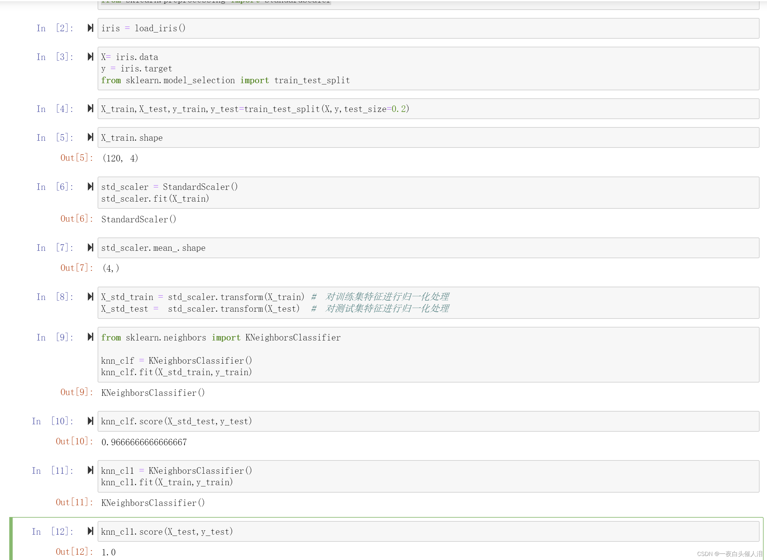
三、鸢尾花数据归一化

import numpy as np
from sklearn.datasets import load_iris
from sklearn.preprocessing import StandardScaler

iris = load_iris()
X= iris.data
y = iris.target
from sklearn.model_selection import train_test_split
X_train,X_test,y_train,y_test=train_test_split(X,y,test_size=0.2)
X_train.shape
std_scaler = StandardScaler()
std_scaler.fit(X_train)
std_scaler.mean_.shape
X_std_train = std_scaler.transform(X_train) #  对训练集特征进行归一化处理
X_std_test =  std_scaler.transform(X_test)  #  对测试集特征进行归一化处理

from sklearn.neighbors import KNeighborsClassifier

knn_clf = KNeighborsClassifier()
knn_clf.fit(X_std_train,y_train)
knn_clf.score(X_std_test,y_test)
knn_cl1 = KNeighborsClassifier()
knn_cl1.fit(X_train,y_train)
knn_cl1.score(X_test,y_test)

四、knn算法总结

#  knn： 天然可以解决分类的算法
#        思想简单，效果强大
#  缺点： 效率很低 
#  缺点： 高度数据相关outlier
#  缺点： 预测的结果不具有可解释性
#  缺点： 维数灾难： 随着维度的增加，看似很相近的点，之间的距离会越来越大

五、线性回归

#  线性回归：判断数据的特征和目标值之间具有一定的线性关系
#  最简单的线性回归：样本的特征只有一个，用线性回归法进行预测，叫做简单线性回归
#  推广到样本特征有多个，多元线性回归
#  实现简单，是很多非线性模型的基础
#  结果具有很强的解释性，可以学习到一些真实世界中的知识
#   np.sum(|y` - y| )
#   np.sum(（y` - y）**2）
#   损失函数

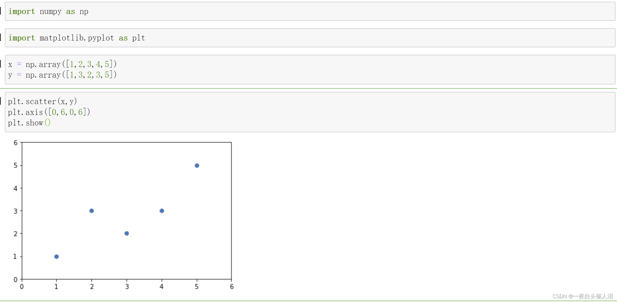
import numpy as np
import matplotlib.pyplot as plt
x = np.array([1,2,3,4,5])
y = np.array([1,3,2,3,5])
plt.scatter(x,y)
plt.axis([0,6,0,6])
plt.show()

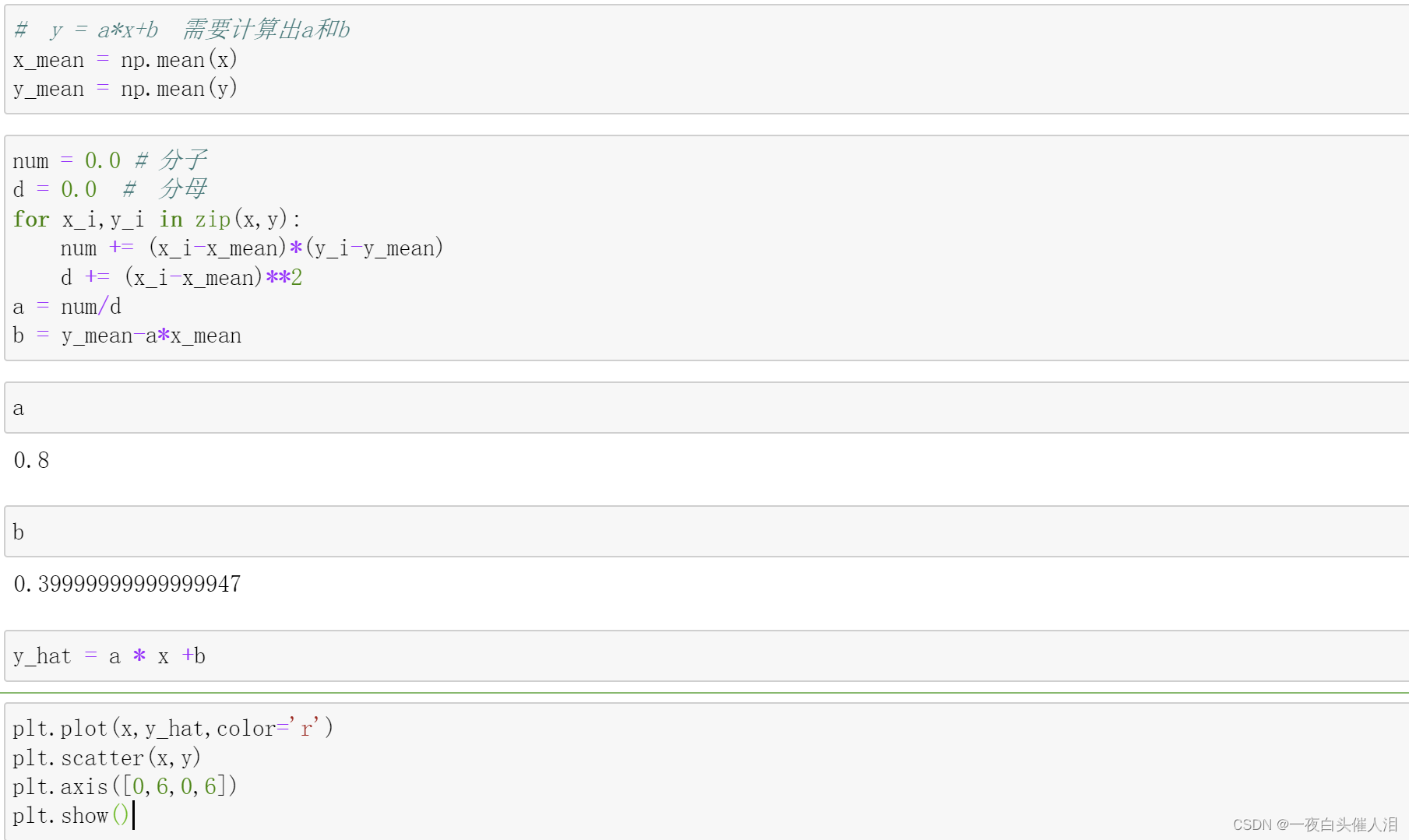
#  y = a*x+b  需要计算出a和b
x_mean = np.mean(x)
y_mean = np.mean(y)
num = 0.0 # 分子
d = 0.0  #  分母
for x_i,y_i in zip(x,y):
    num += (x_i-x_mean)*(y_i-y_mean)
    d += (x_i-x_mean)**2
a = num/d
b = y_mean-a*x_mean
a
b
y_hat = a * x +b
plt.plot(x,y_hat,color='r')
plt.scatter(x,y)
plt.axis([0,6,0,6])
plt.show()

x_predict = 3.5
a*x_predict+b
%run MechainLearning/SimpleLinearRegression.py
lin_reg = SimpleLinearRegression()
lin_reg.fit(x,y)
lin_reg.predict()

SimpleLinearRegression.py

import numpy as np


class SimpleLinearRegression:
    def __init__(self):
        self.a_ = None
        self.b_ = None
        self.x_mean = None
        self.y_mean = None

    def fit(self, x_train, y_train):
        self.x_mean = np.mean(x_train)
        self.y_mean = np.mean(y_train)
        num = 0.0  # 分子
        d = 0.0  # 分母
        for x_i, y_i in zip(x_train, y_train):
            num += (x_i - self.x_mean) * (y_i - self.y_mean)
            d += (x_i - self.x_mean) ** 2
        self.a = num / d
        self.b = self.y_mean - self.a * self.x_mean
        return self

    def predict(self, x_test):
        return self.a * x_test + self.b

moduel_selection.py

import numpy as np


def train_test_split(X, y, test_ratio=0.2, random_state=None):
    if random_state:
        np.random.seed(random_state)
    shuffle_indexs = np.random.permutation(len(X))
    test_ratio = test_ratio
    test_size = int(len(X) * test_ratio)

    test_indexs = shuffle_indexs[:test_size]
    train_indexs = shuffle_indexs[test_size:]
    X_train = X[train_indexs]
    y_train = y[train_indexs]


    X_test = X[test_indexs]
    y_test = y[test_indexs]
    return X_train, X_test, y_train, y_test

from sklearn.neighbors import KNeighborsClassifier

knn = KNeighborsClassifier()

draft.py

import random

random.seed(666)
print(random.random())
print(random.random())
print(random.random())

def random(num):
    pass

六、简单线性回归

# 前提：认为数据具有一定的线性关系
#  希望找到一条最佳拟合的直线方程，只针对简单线性回归（只有一个特征值）
#  y = ax+b    对于每一个样本点，在这个直线方程上都有一个预测值，预测值和真实值有一定的差距
#   我们希望这些样本到直线方程的差距之和最小

#  如何计算这些差距？  |y-y~|   sqrt((y-y~)**2)
#  loss function 损失函数  希望损失函数达到最小值

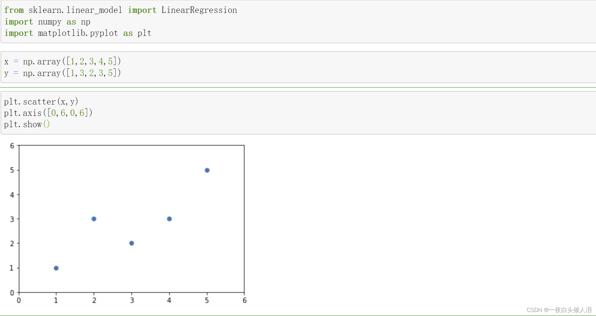
from sklearn.linear_model import LinearRegression
import numpy as np
import matplotlib.pyplot as plt
x = np.array([1,2,3,4,5])
y = np.array([1,3,2,3,5])
plt.scatter(x,y)
plt.axis([0,6,0,6])
plt.show()

lin_reg = LinearRegression()
lin_reg.fit(x.reshape(-1,1),y)
lin_reg.coef_ # 系数
lin_reg.intercept_  # 截距
plt.scatter(x,y)
plt.plot(x,lin_reg.predict(x.reshape(-1,1)),color='r')
plt.axis([0,6,0,6])
plt.show()

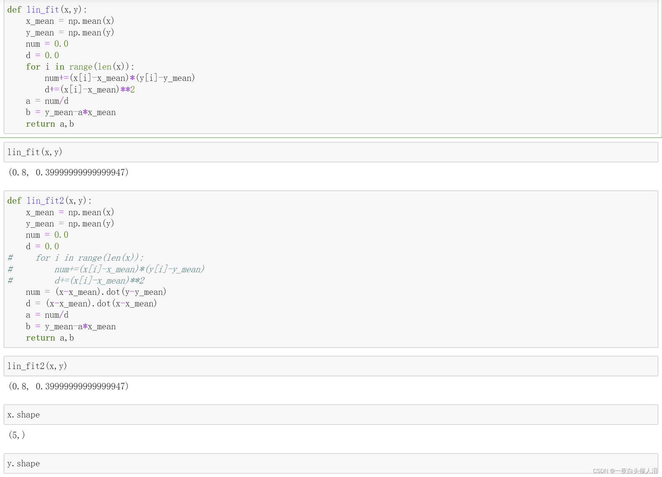
def lin_fit(x,y):
    x_mean = np.mean(x)
    y_mean = np.mean(y)
    num = 0.0
    d = 0.0
    for i in range(len(x)):
        num+=(x[i]-x_mean)*(y[i]-y_mean)
        d+=(x[i]-x_mean)**2
    a = num/d
    b = y_mean-a*x_mean
    return a,b

lin_fit(x,y)

def lin_fit2(x,y):
    x_mean = np.mean(x)
    y_mean = np.mean(y)
    num = 0.0
    d = 0.0
#     for i in range(len(x)):
#         num+=(x[i]-x_mean)*(y[i]-y_mean)
#         d+=(x[i]-x_mean)**2
    num = (x-x_mean).dot(y-y_mean)
    d = (x-x_mean).dot(x-x_mean)
    a = num/d
    b = y_mean-a*x_mean
    return a,b

lin_fit2(x,y)
x.shape
y.shape

七、线性回归模型评优

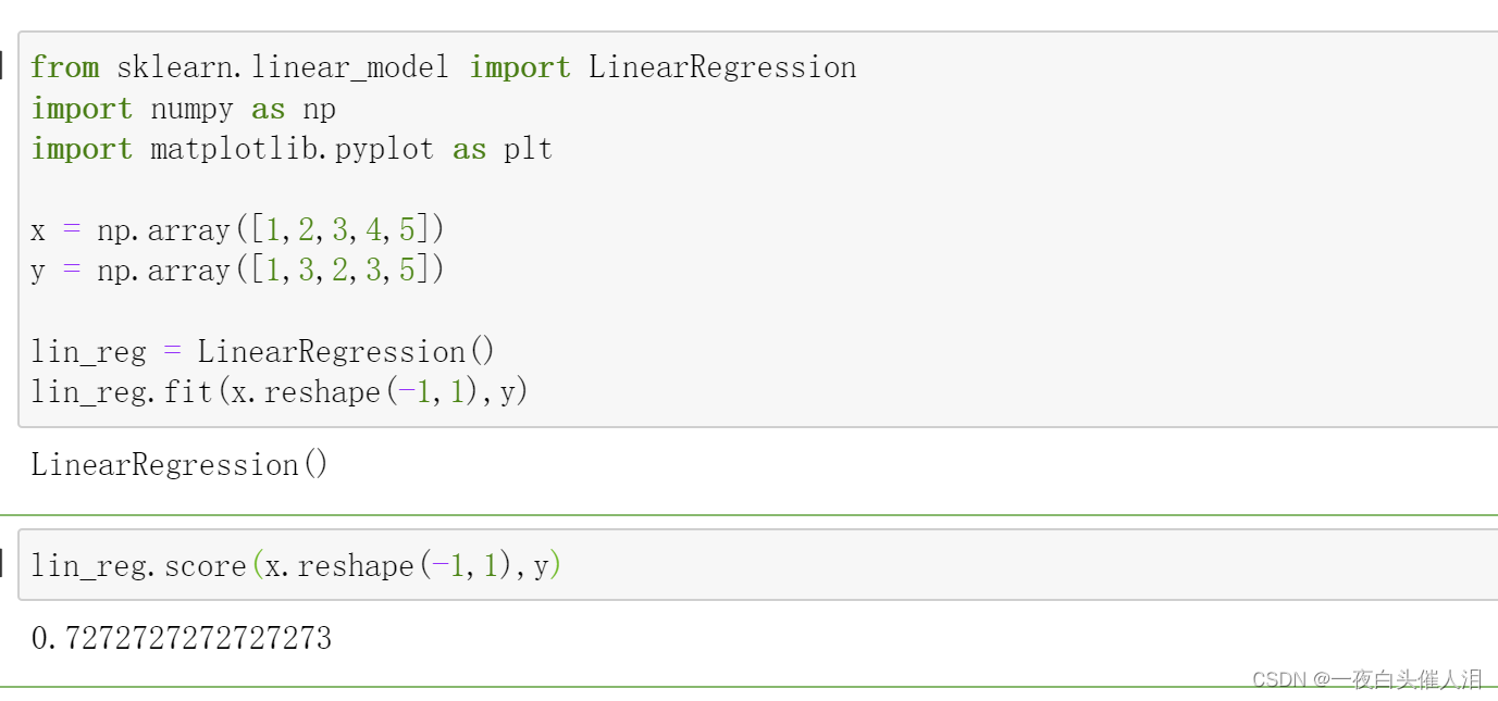
from sklearn.linear_model import LinearRegression
import numpy as np
import matplotlib.pyplot as plt

x = np.array([1,2,3,4,5])
y = np.array([1,3,2,3,5])

lin_reg = LinearRegression()
lin_reg.fit(x.reshape(-1,1),y)

lin_reg.score(x.reshape(-1,1),y)

线性回归模型中的误差计算

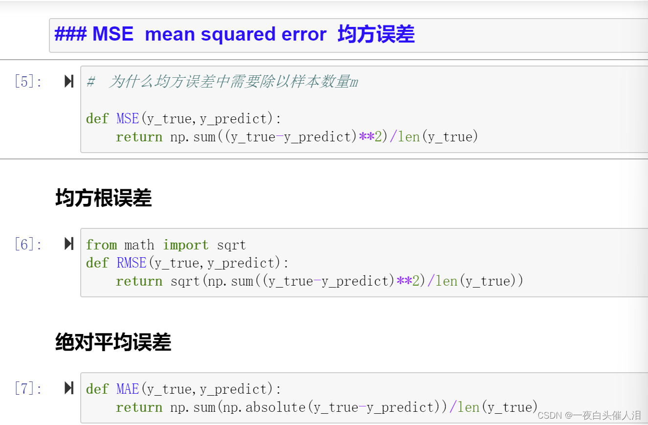
MSE mean squared error 均方误差

#  为什么均方误差中需要除以样本数量m 

def MSE(y_true,y_predict):
    return np.sum((y_true-y_predict)**2)/len(y_true)

均方根误差
from math import sqrt
def RMSE(y_true,y_predict):
    return sqrt(np.sum((y_true-y_predict)**2)/len(y_true))

绝对平均误差
def MAE(y_true,y_predict):
    return np.sum(np.absolute(y_true-y_predict))/len(y_true)

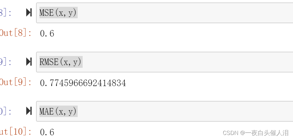
MSE(x,y)
RMSE(x,y)
MAE(x,y)

from sklearn.metrics import mean_squared_error,mean_absolute_error
mean_squared_error(x,y)
mean_absolute_error(x,y)
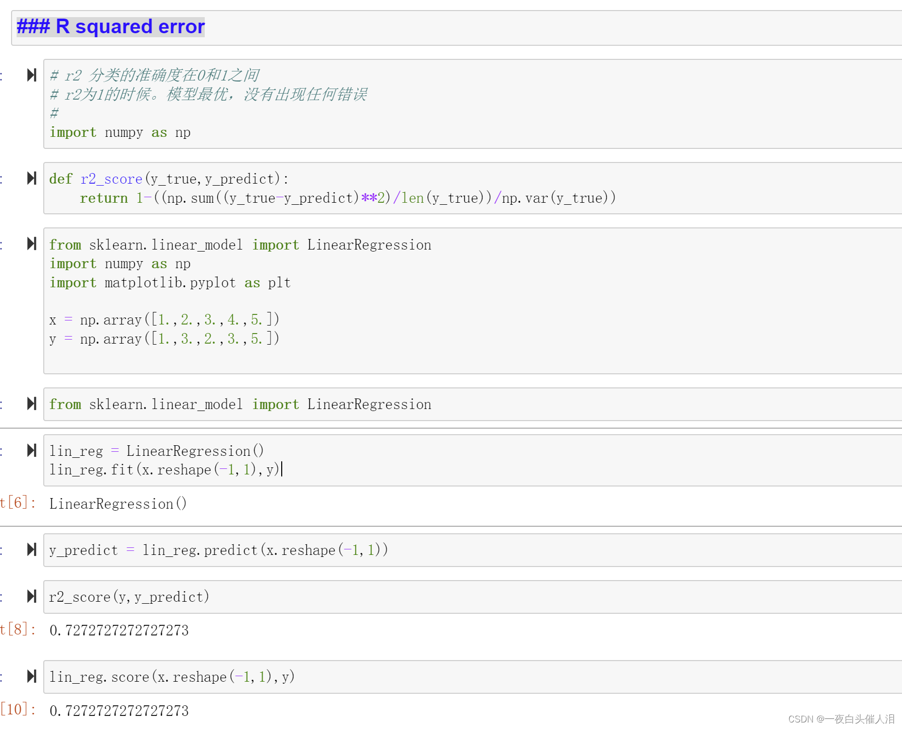
def r2_score(y_true,y_predict):
    return 1-MSE(y_true,y_predict)/np.var(y_true)
r2_score(x,y)

R squared error

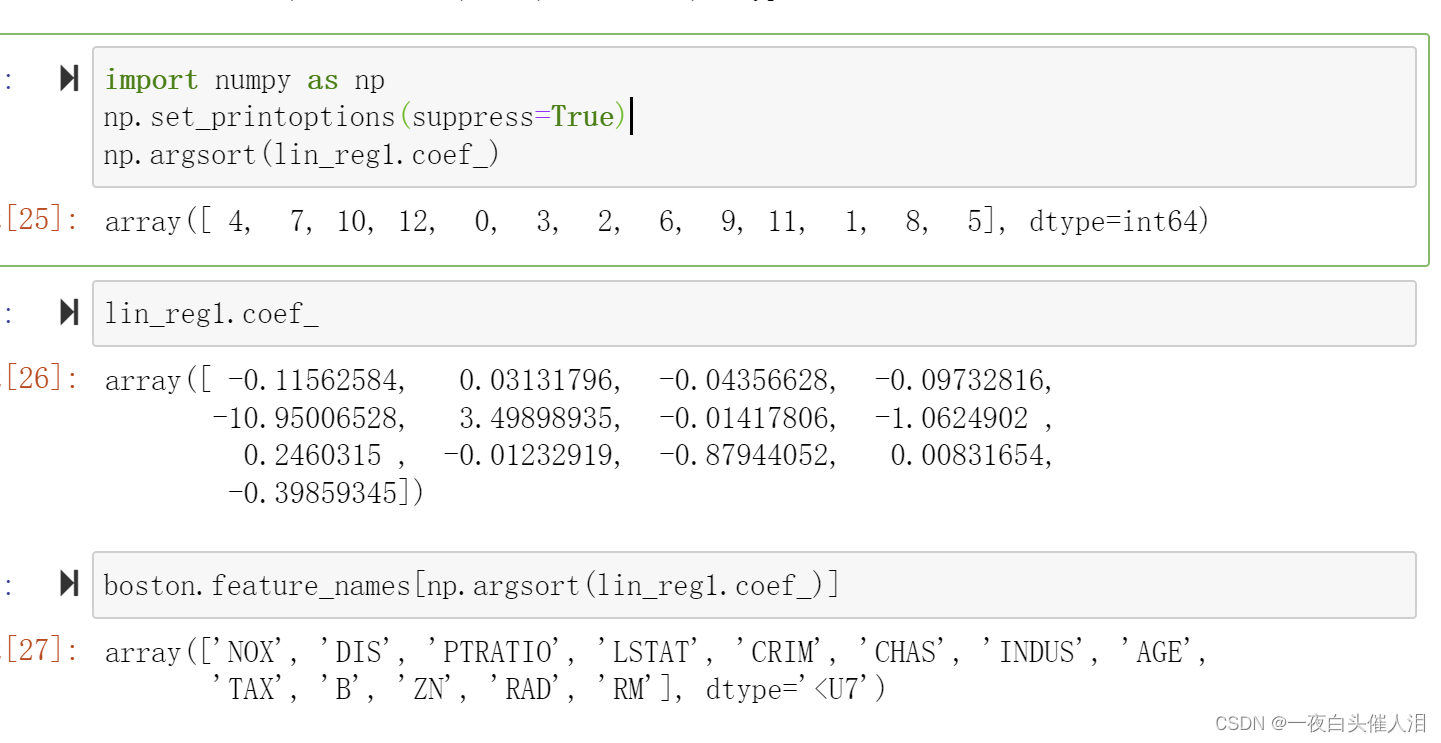
八、多线线性回归

# 特征值不止一个，叫做多元线性回归
#  通过对矩阵进行转换，加一个x0维度，可以得到求出两个矩阵点乘的最小值问题
#  得到西塔的正规方程解，带入x和y就可以求出西塔
#  西塔是一个n+1 * 1 的矩阵
#  西塔0代表截距，西塔除第一个以外的元素代表系数

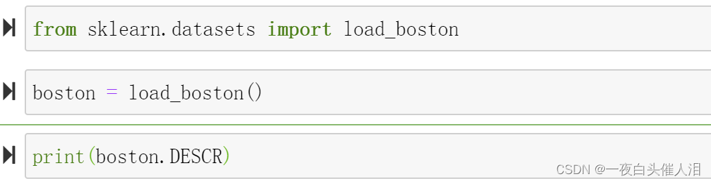
from sklearn.datasets import load_boston
boston = load_boston()
print(boston.DESCR)

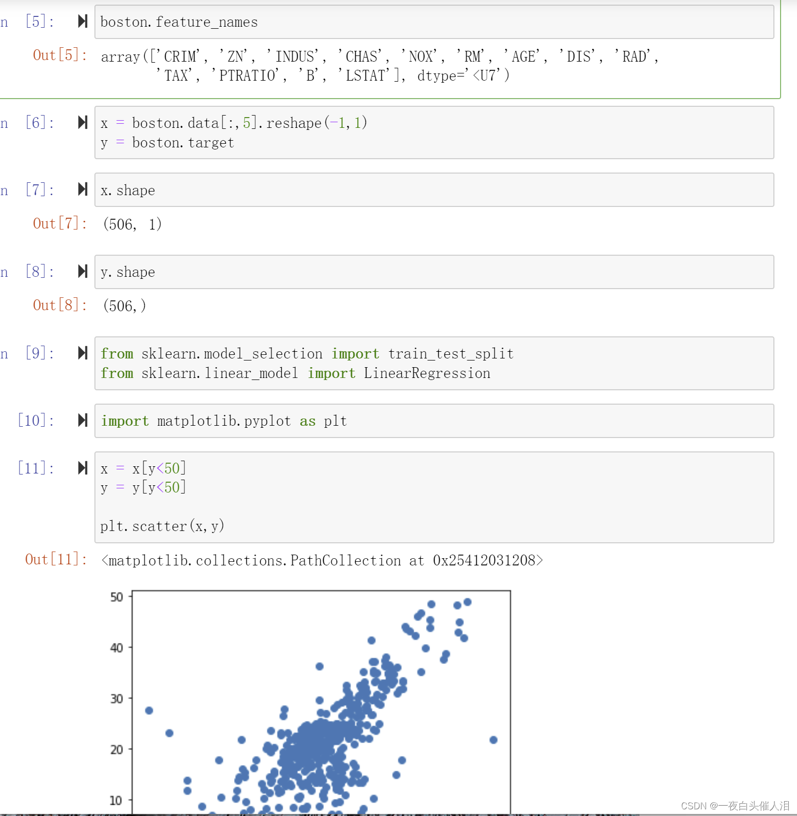
boston.feature_names
x = boston.data[:,5].reshape(-1,1)
y = boston.target
x.shape
y.shape
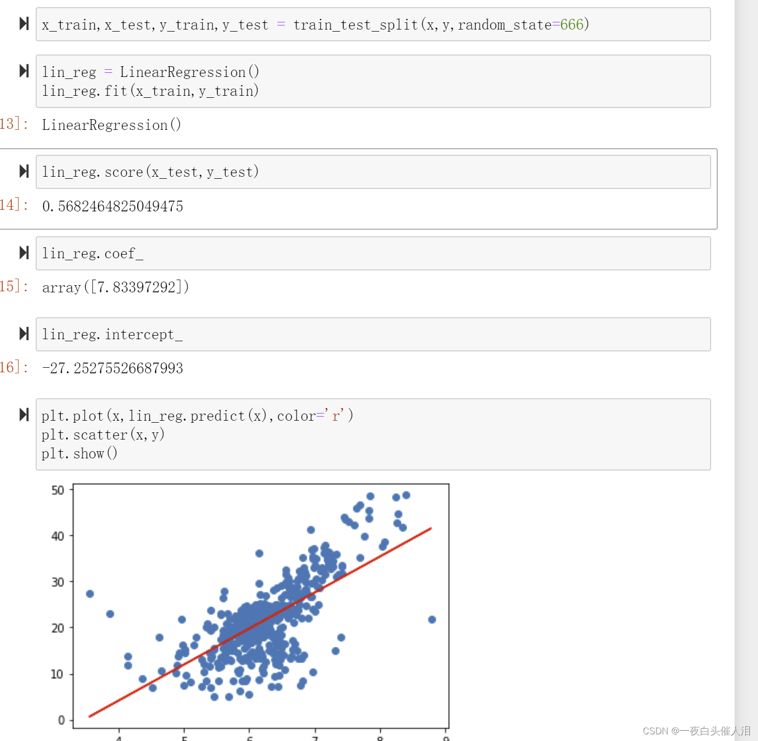
from sklearn.model_selection import train_test_split
from sklearn.linear_model import LinearRegression
import matplotlib.pyplot as plt
x = x[y<50]
y = y[y<50]

plt.scatter(x,y)

from spectral import *
from scipy.io import loadmat#读取数据并显示
input_image = loadmat('dc.mat')['imggt']
input_image_gt = loadmat('dc.mat')['imggt'][1,:,:] 
v = imshow(input_image_gt)
v1 = imshow(input_image)
# principal_components计算图像数据的主组件，并返回一个主组件中的平均值、协方差、特征值和特征向量
pc = principal_components(input_image)
v2 = imshow(pc.cov)
#显示协方差矩阵 白色 强正协方差，深色 强负协方差，灰色 协方差接近于0
#保留至少99.9%的总图像方差
pc_0999 = pc.reduce(fraction = 0.99)
pc_0999.eigenvalues
#获取特征值
len(pc_0999.eigenvalues)#特征值数组长度为270
img_pc = pc_0999.transform(input_image)
v = imshow(img_pc[:,:,:3],stretch_all = True)